3 Alternative notations
3.1 Geometric interpretation
|
1676
|
In 1676, Abraham de Moivre (1667-1754) stated his useful theorem.
He concluded this without using a graphical representation of complex numbers on a plane.
|
|
De Moivre
|
\(\left(\cos{\alpha}+i\sin{\alpha}\right)^n=\cos{n\alpha}+i\sin{n\alpha}\)
|
Eq. 1
|
When we first look at the geometric aspects of complex numbers, it is easy to deduce the theorem.
The theorem is therefore resumed 3.1.4.
|
1702
1748
|
A legion of geniuses was needed to get from the first insights about complex logarithms in 1702 to the famous formula of Euler in 1748.
(Wikipedia - Euler's formula, sd)
|
|
Euler ' formula
|
\(\left(\cos{\alpha}+i\sin{\alpha}\right)^\ =\ e^{i\alpha}\)
|
Eq. 2
|
Euler's formula is addressed in 3.2.
|
1797
|
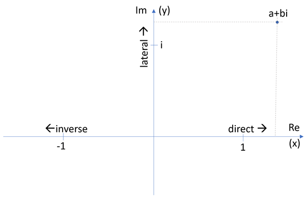
In 1797 John Wagner was the first to draw complex numbers on a plane with a real and an imaginary axis. The fact that Descartes, the man associated with coordinate systems, did not come up with this idea, shows this step is not trivial. (Wikipedia - Euler's formula, sd) (Merino, 2006)
|
Showing a \(a+bi\) on a real and imaginary axis is not shocking.
The leap forward occurs when the effect of operations is visualized on the plane.
3.1.1 Choice of a norm
In mathematics, a norm can be chosen.
Choosing \(\|a+bi\|=\sqrt{a^2+b^2}\) is appropriate in the context of this document.
The norm\(\sqrt{a^2+b^2}\)is the distance from the origin\(\ 0+0i\) to the number \(a+bi\) in the complex plane.
It is often useful to convert complex numbers into the format below:
|
|
\(a+bi=\ \sqrt{a^2+b^2}\left(\cos{\alpha}+i\sin{\alpha}\right)\ where\ \alpha=atan2{(b,a)}\)
|
Eq.3
|
The step towards a polar representation of a complex number is therefore trivial.
|
|
\(a+bi\ \equiv\ r\left(\cos{\alpha}+i\sin{\alpha}\right)\ \equiv\ r\angle\alpha\ \ where\ r=\sqrt{a^2+b^2}\)
\(and\ \alpha=atan2{\left(b,a\right)}\)
\(r\) is called modulus and \(\alpha\ \)the argument
\(r\angle\alpha\equiv"modulus"\angle"argument"\)
|
Eq.4
|
Eq.3 is a little more compact:
|
|
\(a+bi=\ r\left(\cos{\alpha}+i\sin{\alpha}\right)\ with\ r=\sqrt{a^2+b^2}\ en\ \ \alpha=atan2{(b,a)}\)
|
Eq.5
|
This is visualized in Figure 4 for the number \(z_1=1+1i\ \)or \(\sqrt2\ \angle\frac{\pi}{4}\)
|

|
|
Figure 4: Geometric representation of a complex number (GeoGebra)
|
3.1.2 Multiplication
Using the above the following results for the multiplication of two complex numbers:
|
|
\(a+bi=\ r_1\left(\cos{\alpha}+i\sin{\alpha}\right)\ with\ r_1=\sqrt{a^2+b^2}\ \)
\(and\ \ \alpha=atan2{(b,a)}\)
\(c+di=\ r_2\left(\cos{\beta}+i\sin{\beta}\right)\ with\ r_1=\sqrt{c^2+d^2}\)
\(and\ \ \beta=atan2{(d,c)}\)
|
Eq.6
|
Multiplying the 2 binomials:
|
|
|
\(\left(a+bi\right)\left(c+di\right)\)
\({=r}_1\left(\cos{\alpha}+i\sin{\alpha}\right)r_2\left(\cos{\beta}+i\sin{\beta}\right)\)
\({=r}_1r_2\left(\left(\cos{\alpha}\cos{\beta}-\sin{\alpha}\sin{\beta}\ \right){+\ i\ \left(\cos{\alpha}\sin{\beta}+\sin{\alpha}\cos{\beta}\right)}\right)\)
\({=r}_1r_2\left(\cos{\left(\alpha+\beta\right)}{+\ i\ \sin{\left(\alpha+\beta\right)}}\right)\)
\({=r}_1r_{2\ }\angle\alpha+\beta\)
|
Eq.7
|
3.1.3 Beware!
|
In the context of this document: \(r\angle\theta\equiv\ r\ \left(\cos{\theta}+i\sin{\theta}\right)\ \in\mathbb{C}\), so \(r\angle\theta\in\mathbb{C}\).
\(\left(r,\ \theta\right)\in\ \mathbb{R}^2\)is not an alternative representation of a complex number,
it is an alternative representation of a point\(\left(x,y\right)\in\ \mathbb{R}^2\)
|
3.1.4 De Moivre
Now we take the formula of De Moivre:
|
De Moivre
|
\(\left(\cos{\alpha}+i\sin{\alpha}\right)^n=\cos{\left(n\alpha\right)}+i\sin{\left(n\alpha\right)}\)
|
(Eq. 1)
|
|
|
\(\left(1\angle\alpha\right)^n=\ 1^n\angle\left(n\alpha\right)\)
|
|
Intuitively De Moivre can be deduced from Eq.7.
|
|
\(\left(\cos{\alpha}+i\sin{\alpha}\right)^n=\ \left(1\angle\alpha\right)^n=\left(1\angle\alpha\right)\ \left(1\angle\alpha\right)\ldots\ \left(1\angle\alpha\right)\)
\(\ 1^n\angle\left(n\alpha\right)=\cos{\left(n\alpha\right)}+i\sin{\left(n\alpha\right)}\)
|
Eq. 8
|
On (Wikipedia - De Moivre's formula, sd) the theorem is proven by induction, which is a formalization of Eq. 8.
3.2 Eulerian notation
3.2.1 Introduction
|
1748
|
In 1748, Euler proved:
|
|
Euler's Formula
|
\(\left(\cos{\alpha}+i\sin{\alpha}\right)^\ =\ e^{i\alpha}\)
|
(Eq. 2)
|
Purely mathematically, proving the correctness of Euler's formula is not difficult.
The question in this document is what formulation, reasoning or proof creates a (sense of) insight.
|
1800
|
Creating an intuitive understanding of complex numbers is not trivial.
A statement by a 19th-century mathematician, Benjamin Pierce, illustrates this:
"It is Absolutely Paradoxical; we cannot understand it, and we don't know what it means, but we have proved It,
and therefore we know it must be the truth." (Wikiquote - Euler's identity, sd).
|
3.2.1.1 \(\left(cos{\alpha}+isin{\alpha}\right)^\ \rightarrow\ e^{i\alpha}\)
In this document, five different reasonings are elaborated, all leading to the Eulerian representation of complex numbers.
Each reasoning has a different starting point:
1. Powers of \(i\)
2. Powers of \(-1\)
3. Taylor-Series
4. Powers of a complex number\(\ 1+bi\)
5. De Moivre
These reasonings start from the knowledge or an expectation that a complex number can be written as a power of \(e\) and seek a logical path from \(\left(\cos{\alpha}+i\sin{\alpha}\right)^\ \)to \(e^{i\alpha}\) .
The reasoning 'powers of \(i\)' seems to create the best intuitive insight and is therefore elaborated in 3.2.2.
The four other reasonings are included in the Appendix 7.3.
The reasoning 'powers of \(i\)' leads to the core insight of this document:
|
a. Raising \(i\) to a natural power \(n\) is rotating over\(\ n\frac{\pi}{2}\ of\ n90° \) starting from \(i^0=1+0i\).
b. Raising \(i\) to a real power\(\ \theta\frac{2}{\pi}\), corresponds with a rotation over an angle \(\theta\frac{2}{\pi}\ \theta\ \) starting from \(i^0=1+0i\).
|
|
c. A power of a number can always be forced into a power of \(e,\)
using the property \(a^y=\ \ e^{yln{a}}\)
Because a rotation in the complex plane can be written as a power of \(i\), a rotation in the complex plane can be written as a power of \(e\).
|
3.2.1.2 \({Differential\ Equation\ \rightarrow\ e}^{i\alpha}\rightarrow\ f{\left(\alpha\right)}\)
An alternative path rolls out the search for solutions of linear differential equations.
When looking for a solution to a differential equation, \(e\) pops up in a natural way.
From there a real-valued function must be found corresponding to that solution.
This is elaborated in 7.2
3.2.2 From the powers of \(i\) to \(e^{i\alpha}\)
In 2.56 it was observed that multiplication of a complex number by \(i\) corresponds to rotation over \(\frac{\pi}{2}\) on the complex plane.
We observe that a natural power of a complex number corresponds to a linear growth of the angle.
|
|
\(i=0+1i=\ 1\left(\cos{\left(\frac{\pi}{2}\right)}+i\ \sin{\left(\frac{\pi}{2}\right)}\right)=1\angle\frac{\pi}{2}\)
|
Eq. 9
|
|
De Moivre
|
\(\left(\cos{\alpha}+i\sin{\alpha}\right)^n=\cos{n\alpha}+i\sin{n\alpha}\)
|
(Eq. 1)
|
Applying De Moivre to Eq. 9 provides:
|
|
\(i^n=1\left(\cos{\left(n\frac{\pi}{2}\right)}+i\ \sin{\left(n\frac{\pi}{2}\right)}\right)=1\angle\left(n\frac{\pi}{2}\right)\ ,\ n\in\mathbb{N}\)
|
Eq. 10
|
|
What happens if we raise \(i\) to a real (\(\in\mathbb{R}\)) power instead of a natural \(\left(\in\mathbb{N}\right)\)power?
|
Extending Eq. 10 to \(\mathbb{R}\) results in:
|
|
\(i^x=1\left(\cos{\left(x\frac{\pi}{2}\right)}+i\ \sin{\left(x\frac{\pi}{2}\right)}\right)=1\angle\left(x\frac{\pi}{2}\right)\ ,\ x\in\mathbb{R}\)
|
Eq. 11
|
|
|
\(i^{\theta\frac{2}{\pi}}=1\left(\cos{\theta}+i\ \sin{\theta}\right)=1\angle\theta\ \ x,\ \theta\in\mathbb{R},\ \theta=x\ \frac{\pi}{2}\)
|
Eq. 12
|
We no longer rotate in discrete steps \(n\in\mathbb{N}\), but over ‘any angle’ \(\theta\).
|
Raising \(i\) to a real power \(\theta\frac{2}{\pi}\ \), corresponds to a rotation over an angle \(\theta\) from \(i^0=1+0i\ or\ 1\angle0\).
Now we can rotate over any angle \(\theta\) on the complex plane.
|
|
|
\(a^y=\ \left(e^{\ln{a}}\right)^y=\ \ e^{y\ln{a}}\)
|
(Eq. 73)
|
|
A power of any number, including \(i\), can be rewritten as a power of \(e.\)
|
Using Eq. 73:
|
|
\(i^{\theta\frac{2}{\pi}}=\ e^{\ln{\left(i\right)\theta\frac{2}{\pi}}}\)
|
Eq. 13
|
|
|
\(i^{\theta\frac{2}{\pi}}=\ e^{\ln{\left(i\right)\theta\frac{2}{\pi}}}=\ 1\left(\cos{\theta}+i\ \sin{\theta}\right)\)
|
Eq. 14
|
|
|
\(i^{\theta\frac{2}{\pi}}=\ e^{\ln{\left(i\right)\theta\frac{2}{\pi}}}=\ 1\left(\cos{\theta}+i\ \sin{\theta}\right)\)
|
(Eq. 14)
|
In 7.1 Eq. 58 was derived.
|
|
\(\frac{d}{dx}\left(\cos{x}+i\ \sin{x}\right)=i\ \left(\cos{x}+i\sin{x}\right)\)
|
(Eq. 58)
|
|
|
\(\frac{d}{dx}e^{kx}=ke^{kx}\ \)
|
(Eq. 59)
|
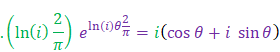
If we take the derivative to \(\theta\) from either side of Eq. 14:
|
|
|
Eq. 15
|
|
|
.\(\left(\ln{\left(i\right)\frac{2}{\pi}}\right)\ e^{\ln{\left(i\right)\theta\frac{2}{\pi}}}=i\left(\cos{\theta}+i\ \sin{\theta}\right)\)
|
|
So:
|
|
\(\left(\ln{\left(i\right)\frac{2}{\pi}}\right)\ \)=\(i\)
|
Eq. 16
|
|
|
\(\ln{\left(i\right)}\ \)=\(i\frac{\pi}{2}\)
|
Eq. 17
|
Combining Eq. 13 and Eq. 17 results in:
|
|
\(i^{\theta\frac{2}{\pi}}=\ e^{\ln{\left(i\right)\theta\frac{2}{\pi}}}\)=\(e^{i\frac{\pi}{2}{\theta\frac{2}{\pi}}}=\ e^{i\theta}=\ 1\left(\cos{\theta}+i\ \sin{\theta}\right)\)
|
Eq. 18
|
|
Raising \(i\) to a power \(\theta\frac{2}{\pi}\ \), corresponds with a rotation over an angle \(\theta\) on the complex plane.
A power of any number, including \(i\), can be rewritten as a power of \(e.\)
|
To extend Eq. 18 to 'any complex number', we only need to multiply by \(r\):
|
|
\(r\ i^{\theta\frac{2}{\pi}}=\ r\ e^{\ln{\left(i\right)\theta\frac{2}{\pi}}}=re^{i\frac{\pi}{2}{\theta\frac{2}{\pi}}}=\ re^{i\theta}=\ r\left(\cos{\theta}+i\ \sin{\theta}\right)=a+bi\)
\(waarbij\ r=\sqrt{a^2+b^2}\ en\ \ \theta=atan2{(b,a)}\)
|
Eq. 19
|
|
Conclusion: Any complex number\(\ a+bi\) can be written as \({re}^{i\theta}\).
|
3.2.3 Euler's identity
In Eq. 19 we substitute \(r=1\ \)and \(\theta=\pi\)
|
|
\({re}^{i\pi}=\ r\left(\cos{\pi}+i\sin{\pi}\right)\ \)
|
Eq. 20
|
|
Euler's Identity
|
\(1\angle\pi=\ -1+0i=\ e^{i\pi}\)
\(e^{i\pi}+1=0\)
|
Eq. 21
|
Because Euler's identity contains three basic constants and basic mathematical operations,
it is considered to be the most beautiful formula of mathematics. (Wikiquote - Euler's identity, sd)
3.2.4 Visualization
of \({x+yi=\left(ri\right)}^{at\frac{2}{\pi}}\)
Turning around on the unit circle does not result in a useful representation.
If we now show time \(t\ \)on the third axis, the z-axis, a nice visualization arises.
|
|
|
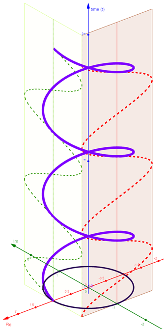
Figure 5:\({x+yi=1\ i}^{3t\frac{2}{\pi}}=1\ e^{iat}=1\angle3t\ \ describes\ a\ \ spiral\ \)(GeoGebra)
|
We choose \(r=1\ \)and\(\ a=3\)in \({x+yi=\left(ri\right)}^{at\frac{2}{\pi}}=\ \ \left(re^{i\alpha}\right)^t=\left(r\angle a\right)^t\).
With\(\ r=1\) the radius, the modulus, remains equal to 1.
\({x+yi=1\ i}^{3t\frac{2}{\pi}}={1\ e}^{i3t}=1\angle3t\ \)rotates over the unit circle with a fixed angular velocity.
If we show time on the z-axis, a beautiful spiral shows.
If the spiral is projected on a plane perpendicular to the Real-axis, a cosine emerges.
The projection on a plane perpendicular to Imaginary axis shows a sine.
4 Complex numbers as a function of time
4.1 (Co)sine-shaped time function
A periodic function that repeats \(f\ \)times a second has a frequency of \(f\ \)expressed in \(Hz\ or\ \frac{1}{s}\).
One period of the function takes \(T\ =\ \frac{1}{f}\ \)second.
When signals are described by sines and/or cosines, then the angle θ runs from \(0\) to \(2\pi\ \)in \(T\)seconds.
The angle θ is called the phase of the time function.
If any time \(t\ \)expires, the angle \(\theta\ \) will have run from \(0\) to \(\frac{2\pi}{T}\ t\) or \(\left(2\pi f\right)t.\)
|
Convention
|
\(\omega=2\pi\ f=\ \frac{2\pi}{T}\)= Angular Velocity
|
Eq. 22
|
If any time \(t\ \)expires, the angle \(\theta\ \) will have run from \(0\) to \(\frac{2\pi}{T}\ t\) or \(\omega\ t.\)
The angle θ can start from a value other than \(0\) too.
This initial angle is called phase shift, often indicated with the letter \(\varphi\).
The value of the function \(\sin{\left(\omega t+\varphi\right)}\) varies between -1 and + 1.
To describe functions with other values, a scale factor, the amplitude \(A\), is added to the description.
A complete description of a (co)sine-shaped time function looks like:
|
Convention
|
\(f{\left(t\right)=A}\sin{\left(\omega t+\varphi\right)}met\ \omega=2\pi\ f=\ \frac{2\pi}{T}\)
|
Eq. 23
|
When describing physical systems, the amplitude\(\ A\) often is a function of time\(\ A\left(t\right)\) too.
In many physical systems, the amplitude is described by a real exponential function:
|
|
\(A\left(t\right)=\ A_0\ \ e^{at}\)
|
Eq. 24
|
|
|
\(f{\left(t\right)=A_0\ \ e^{at}}\sin{\left(\omega t+\varphi\right)}met\ \omega=2\pi\ f=\ \frac{2\pi}{T}\)
|
Eq. 25
|
4.2 Complex-valued time function
|
|
\(f{\left(t\right)=A_0\ \ e^{at}}\sin{\left(\omega t+\varphi\right)}met\ \omega=2\pi\ f=\ \frac{2\pi}{T}\)
|
(Eq. 25)
|
|
|
\({re}^{i\theta}=a+bi=\ r\left(\cos{\theta}+i\sin{\theta}\right)\ \)
\(waarbij\ r=\sqrt{a^2+b^2}\ en\ \ \theta=\arctan{\frac{b}{a}}\)
|
(Eq. 97)
|
From the formula of De Moivre, the following can be deduced:
|
|
\(\cos{\theta}=\ \frac{\left(e^{i\theta}+e^{-i\theta}\right)}{2}\)
|
Eq. 26
|
|
|
\(\sin{\theta}=\ \frac{\left(e^{i\theta}-e^{-i\theta}\right)}{2i}\)
|
|
With \(\theta=\ \omega\ t+\varphi:\)
|
|
\(\cos{\left(\omega t+\varphi\right)}=\ \frac{\left(e^{i\left(\omega t+\varphi\right)}+e^{-i\left(\omega t+\varphi\right)}\right)}{2}\)
|
Eq. 27
|
|
|
\(\sin{\left(\omega t+\varphi\right)}=\ \frac{\left(e^{i\left(\omega t+\varphi\right)}-e^{-i\left(\omega t+\varphi\right)}\right)}{2i}\)
|
|
|
|
\(f{\left(t\right)}=A{\left(t\right)}\cos{\left(\omega t+\varphi\right)}=\ \frac{\left(e^{i\left(\omega t+\varphi\right)}+e^{-i\left(\omega t+\varphi\right)}\right)}{2}\)
|
Eq. 28
|
Using Eq. 24:
|
|
\(f{\left(t\right)}=A_0\ \ e^{at}\cos{\left(\omega t+\varphi\right)}=A_0\ \ e^{at}\ \frac{\left(e^{i\left(\omega t+\varphi\right)}+e^{-i\left(\omega t+\varphi\right)}\right)}{2}\)
|
Eq. 29
|
Substituting:
|
|
\(g{\left(t\right)}=A_0\ \ e^{at}{e^{i\left(\omega t+\varphi\right)}}\)
|
Eq. 30
|
|
|
\(f{\left(t\right)}=A_0\ \ e^{at}\cos{\left(\omega t+\varphi\right)}=\ \frac{g\left(t\right)+\ g^\ast(t)}{2}\)
|
Eq. 31
|
|
|
\(g{\left(t\right)}=A_0\ {e^{at+i\left(\omega t+\varphi\right)}}\)And\(g^\ast(t)=A_0\ {e^{at-i\left(\omega t+\varphi\right)}}\)
|
|
|
|
\(g{\left(t\right)}=A_0e^{i\left(\omega t\right)}\ \ e^{at}{e^{i\left(\omega t\right)}}\)
|
|
|
|
\(g{\left(t\right)}=A_0e^{i\varphi}\ \ e^{at}{e^{i\left(\omega t\right)}}\)
|
|
|
|
\(g{\left(t\right)}=A_0e^{i\varphi}\ \ e^{at+i\omega t}\)
|
|
|
|
\(g{\left(t\right)}=A_0e^{i\varphi}\ \ e^{\left(a+i\omega\right)t}\)And\(g^\ast(t)=A_0e^{-i\varphi}\ e^{\left(a-i\omega\right)t}\)
|
Eq. 32
|
|
|
\(f{\left(t\right)}=A_0\ \ e^{at}\cos{\left(\omega t+\varphi\right)}=\ \frac{g\left(t\right)+\ g^\ast(t)}{2}\)
|
(Eq. 31)
|
Summary:
|
|
\(f{\left(t\right)}=A_0\ \ e^{at}\cos{\left(\omega t+\varphi\right)}=\ \frac{g\left(t\right)+\ g^\ast(t)}{2}\)
|
(Eq. 31)
|
|
|
\(g{\left(t\right)}=A_0e^{i\varphi}\ \ e^{\left(a+i\omega\right)t}\)and\({\ g}^\ast(t)=A_0e^{-i\varphi}\ e^{\left(a-i\omega\right)t}\)
|
(Eq. 32)
|
Eq. 32 allows calculations without getting stuck in trigonometric formulas for sums, products, powers, and derivatives.
The results of calculations based on the format of Eq. 32, can then possibly be converted back to the cosine form.
Eq. 30 can be written in a more compact way as:
|
|
\(g{\left(t\right)}=A\ \ e^{\left(a+i\omega\right)t}\ en\ g^\ast\left(t\right)=A^\ast\ e^{\left(a-i\omega\right)t}\)
\(met\ A=A_0e^{i\varphi}\ en\ \ A^\ast=A_0e^{-i\varphi}\)
|
Eq. 33
|
|
|
\(f{\left(t\right)}=A_0\ \ e^{at}\cos{\left(\omega t+\varphi\right)}=\ \frac{g\left(t\right)+\ g^\ast(t)}{2}\)
|
(Eq. 31)
|
In this notation, one should always be aware that A is a complex number.
It contains both the initial amplitude\(A_0\ \)and the phase\(\ \varphi\).
5 Complex numbers and systems
 Thinking about systems and signals using complex numbers has been introduced by Oliver Heaviside (1850-1925).
5.1 Derivation
The webpage (The RC Filter Transfer Function, 2015) clearly describes how the transfer function of an 'RC filter' is calculated.
|

|
|
Figure 6:\(RC\ Low\ Pass\ Filter\)
|
The transfer function of a system describes an output-quantity of the system as a function of an input-quantity.
For the filter, we determine the transfer function between the input voltage \(v_{in}\)and the output voltage \(v_{out}.\)
|
|
\(\frac{v_{out}}{v_{in}}=\ \frac{1}{\left(j\omega RC+1\right)}\ met\ j=\sqrt{-1}\)
|
Eq. 34
|
|
|
\(\frac{V_{out}}{V_{in}}=\ \left(1+j\omega RC\right)^{-1}\)
|
Eq. 35
|
|
|
\(\frac{v_{out}}{v_{in}}=\ \left(1+j\omega RC\right)^{-1}=r\ e^{j\varphi}\)
\(with\ r=\frac{1}{\sqrt{1+\left(\omega RC\right)^2}}\)

|
Eq. 36
|
|
|

|
Eq. 37
|
|
|

|
Eq. 38
|
From Eq. 38 we can derive:
|
|
\(\varphi\left(-\omega\right)=-\varphi\left(\omega\right)\)
|
Eq. 39
|
Now substitute \(v_{in}=\cos{\left(\omega\ t\right)}=\frac{\left(e^{j\left(\omega\ t\right)}+e^{-j\left(\omega\ t\right)}\right)}{2}\)
|
|
\(v_{in}=\cos{\left(\omega\ t\right)}=\frac{\left(e^{j\left(\omega\ t\right)}+e^{-j\left(\omega\ t\right)}\right)}{2}\)
|
Eq. 40
|
|
|
\(v_{in1}=\frac{\left(e^{j\left(+\omega\right)t}\right)}{2}\)
|
Eq. 41
|
|
|
\(v_{in2}=\frac{\left(e^{j\left(-\omega\right)t}\right)}{2}\)
|
Eq. 42
|
|
|
\(v_{out1}=\ \ \frac{e^{j\varphi\left(+\omega\right)}}{\sqrt{1+\left(\omega\ RC\right)^2}}\frac{\left(e^{j\left(+\omega\right)t}\right)}{2}\)
|
Eq. 43
|
|
|
\(v_{out1}=\ \ \frac{e^{j\left(+\omega\ t+\varphi\left(+\omega\right)\right)}}{2\sqrt{1+\left(\omega\ RC\right)^2}}\)
|
Eq. 44
|
|
|
\(v_{out2}=\ \ \frac{e^{j\varphi\left(-\omega\right)}}{\sqrt{1+\left(\omega\ RC\right)^2}}\frac{\left(e^{j\left(-\omega\right)t}\right)}{2}\)
|
Eq. 45
|
|
|
\(v_{out2}\ \ \)
|
\(=\frac{e^{j\varphi\left(-\omega\right)}}{\sqrt{1+\left(\omega\ RC\right)^2}}\frac{\left(e^{j\left(-\omega\right)t}\right)}{2}\)
|
|
|
|
|
\(=\ \ \frac{e^{-j\varphi\left(\omega\right)}}{\sqrt{1+\left(\omega\ RC\right)^2}}\frac{\left(e^{-j\left(\omega\ t\right)}\right)}{2}\)
|
|
|
|
|
\(=\frac{e^{-j\varphi\left(\omega\right)}}{\sqrt{1+\left(\omega\ RC\right)^2}}\frac{\left(e^{-j\left(\omega\ t\right)}\right)}{2}\)
|
|
|
|
\(v_{out2}\ \ \)
|
\(=\frac{e^{-j\left(\omega\ t+\varphi\left(\omega\right)\right)}}{2\sqrt{1+\left(\omega\ RC\right)^2}}\)
|
Eq. 46
|
|
|
\(v_{out}=\ v_{out1}+v_{out2}\)
|
Eq. 47
|
|
|
\(v_{out}=\frac{e^{j\left(\omega\ t+\varphi\left(\omega\right)\right)}}{2\sqrt{1+\left(\omega\ RC\right)^2}}+\frac{e^{-j\left(\omega\ t+\varphi\left(\omega\right)\right)}}{2\sqrt{1+\left(\omega\ RC\right)^2}}\)
|
|
|
|
\(v_{out}=\frac{1}{\sqrt{1+\left(\omega\ RC\right)^2}}\cos{\left(\omega\ t+\varphi\left(\omega\right)\right)}\)
|
Eq. 48
|
5.2 Conclusion
Symmetry
In both the transfer function \(k\)and the (co)sine-shaped signals\(f\), a symmetry is observed:
|
|
\(f{\left(t\right)}=\ g\left(t\right)+\ g^\ast(t)=\ \ g\left(+\omega,t\right)+\ g\left(-\omega,t\right)\)
|
(Eq. 49)
|
|
|
\(k{\left(\omega\right)}=h\left(+\omega\right)+\ h^\ast(+\omega)=\ \ h\left(+\omega\right)+h\left(-\omega\right)\)
|
(Eq. 50)
|
The second part of the sums does not contain any additional information and therefore it does not make any sense to perform the calculations for both members of the sum.
Directly from complex representation to a cosine
If the derivation in 5.1 is reviewed, it can be concluded that the calculation \(v_{out2}\)does not yield any additional information.
This means that when considering a signal and obtaining a result in the format of Eq. 51:
|
|
\(\frac{A}{2}e^{j\ \left(\omega\ t+\varphi\left(\omega\right)\right)}\ met\ A\in\mathbb{R}\)
|
Eq. 51
|
it can always be concluded this corresponds to Eq. 52:
|
|
\(A\cos{\left(\omega t+\varphi\left(\omega\right)\right)}\)
|
Eq. 52
|
Directly from system to complex notation
Conversely, there is no need to start any reasoning on a system from the input signal written in the form of a (co)sine.
One can start immediately in the complex notation, knowing it can, at all times, be converted to a (co)sine.
Directly from transfer function to output signal
Taking Eq. 36:
|
|
\(\frac{v_{out}}{v_{in}}=\ \left(1+j\omega RC\right)^{-1}=r\left(\omega\right)\ e^{j\varphi\left(\omega\right)}\)
\(with\ r\left(\omega\right)=\frac{1}{\sqrt{1+\left(\omega RC\right)^2}}\)
|
(Eq. 36)
|
and Eq. 48:
|
|
\(v_{out}=\frac{1}{\sqrt{1+\left(\omega\ RC\right)^2}}\cos{\left(\omega\ t+\varphi\left(\omega\right)\right)}\)
|
(Eq. 48)
|
It can be concluded that the complete calculation does not need to be carried out and \(v_{out}\)can be derived directly from Eq. 36, if the input signal is a (co)sine.
Periodic non-sine-shaped signals
Most periodic non-sine-shaped signals can be written as a linear combination of sines and/or cosines.
If the input signal \(v_{in}\ \)is a linear combination of (co)sines, the output signal \(v_{out}\ \)is a linear combination of (co)sines too,
where each component \(\cos{\left(\omega t\right)}\) is scaled with \(r\left(\omega\right)\ \)and shifted with \(\varphi\left(\omega\right)\ \)as the transfer function describes.
6 N-the root of a complex number
6.1 Derivation
This derivation is taken from (uhasselt@school - Lesmateriaal - Complexe getallen, sd)
Each number \(z\) that for which \(z^n=w\) holds, is an n-the power root of \(w\).
The above equality can be rewritten as a polynomial.
|
|
\(z^n=w\ {\Longleftrightarrow}z^n-w=\ 0\)
|
Eq. 53
|
|
|
\(y\left(z\right)=\ z^n-w\)
|
Eq. 54
|
The polynomial \(y(z)\)has n zeros.
|
|
\(w=r\ \left(\cos{\alpha}+i\ \sin{\alpha}\right)\)
|
Eq. 55
|
|
|
\(z=\)ρ\(\ \left(\cos{\phi}+i\ \sin{\phi}\right)\)
|
|
Using De Moivre we obtain:
|
|
\(z^n=\rho^n\ \left(\cos{\left(n\phi\right)}+i\ \sin{\left(n\phi\right)}\right)\)
|
|
|
|
\(w=r\ \left(\cos{\alpha}+i\ \sin{\alpha}\right)=\rho^n\ \left(\cos{\left(n\phi\right)}+i\ \sin{\left(n\phi\right)}\right)=z^n\)
|
|
|
|
r =\(\rho^n\ en\ \left(\cos{\alpha}+i\ \sin{\alpha}\right)\)=\(\left(\cos{\left(n\phi\right)}+i\ \sin{\left(n\phi\right)}\right)\)
|
|
For which angle(s) \(\alpha\) does the following hold?
|
|
\(\ \cos{\alpha}=\ \cos{\left(n\phi\right)}\ and\ \ \sin{\alpha}\)=\(\cos{\left(n\phi\right)}\) ?
|
Eq. 56
|
Eq. 57 applies to any\(\ \alpha:\)
|
|
\(\ \alpha=n\phi+k\ 2\pi\)
|
Eq. 57
|
|
|
\(\phi=\frac{\alpha}{n}+k\ \frac{2\pi}{n}\)
|
|
\(z\) is an n-th power root of a complex number \(w=r\ \left(\cos{\alpha}+i\ \sin{\alpha}\right)\ \)if and only if
|
|
\(z=\sqrt[n]{r}\ \left(\cos{\left(\frac{\alpha}{n}+k\ \frac{2\pi}{n}\right)}+i\ \ \sin{\left(\frac{\alpha}{n}+k\ \frac{2\pi}{n}\right)}\right)\)
|
|
6.2 Visualization
We Consider an example where \(r=1\). We are looking for the 5th-roots \(\left(z_1\ldots z_5\right)\ \)of number
|
|
\(w=r\ \left(\cos{\alpha}+i\ \sin{\alpha}\right)=1\ cos60°+i sin60°\)
|
|
|

|
|
Figure 7: Fifth roots \((z_1\)...\(z_5)\ \)of a complex number w (GeoGebra)
|
7 Appendices
7.1 Appendix: n-th derivative of \(cos{x}+isin{x}\)
The derivation is not elaborated, only a consecutive series of derivatives are listed:
|
|
\(\frac{d^n}{dx}\left(\cos{x}+i\sin{x}\right)=i^n\ \left(\cos{\left(x\right)}+i\sin{\left(x\right)}\right)\)
|
Eq. 58
|
|
\(k\)
|
|
\(\frac{d^k}{dx}\)
|
|
\(i^k\ \left(\cos{\left(x\right)}+i\sin{\left(x\right)}\right)\)
|
\(i^k\)
|
Rotation
|
|
0
|
\(+cos(x)\)
|
+ \(i\)
|
\(+sin(x)\)
|
\(+\cos{\left(x\right)}+i\sin{\left(x\right)}\)
|
\(+1\)
|
\(0\)
|
|
1
|
\(-sin(x)\)
|
+ \(i\)
|
\(+cos(x)\)
|
\(-\sin{\left(x\right)}+i\cos{\left(x\right)}\)
|
\(+i\)
|
\(1\frac{\pi}{2}\)
|
|
2
|
\(-cos(x)\)
|
+ \(i\)
|
\(-sin(x)\)
|
\(-\cos{\left(x\right)}-i\sin{\left(x\right)}\)
|
\(-1\)
|
\(2\frac{\pi}{2}\)
|
|
3
|
\(+sin(x)\)
|
+ \(i\)
|
\(-cos(x)\)
|
\(+\sin{\left(x\right)}-i\cos{\left(x\right)}\)
|
\(-i\)
|
\(3\frac{\pi}{2}\)
|
|
4
|
\(+cos(x)\)
|
+ \(i\)
|
\(+sin(x)\)
|
\(+\cos{\left(x\right)}+i\sin{\left(x\right)}\)
|
\(+1\)
|
\(4\frac{\pi}{2}\)
|
|
a. Deriving the expression \(\cos{x}+i\sin{x}\) corresponds to multiplying by\(\ i.\)
b. By multiplying by \(i\), the real part and the imaginary part are always swapped:

c. Successive powers of \(i\) show the same sign changes that arise in the coordinates when a point is rotated over 90 ° or\(\frac{\pi}{2}\):

|
The following expressions illustrate the similarity between exponential and trigonometric functions even more.
|
|
\(\frac{d^n}{dx}\left(\cos{x}+i\sin{x}\right)=i^n\ \left(\cos{\left(x\right)}+i\sin{\left(x\right)}\right)\)
|
|
|
|
\(\frac{d{\ e}^{kx}}{dx}=ke^{kx}\ \Rightarrow\ \frac{d^ne^{kx}}{dx}=k^ne^{kx}\)
|
Eq. 59
|
|
|
\(\frac{{d\ e}^{ix}}{dx}=i\ e^{ix}\ \Rightarrow\ \frac{{d\ e}^{ix}}{dx}=i^ne^{ix}\)
|
|
|
|
\(\frac{d{\ e}^{i\omega\ t}}{dx}=\left(i\omega\right)\ e^{i\omega\ t}\ \Rightarrow\ \frac{d^ne^{i\omega\ t}}{dx}=\left(i\omega\right)^ne^{i\omega\ t}\)
|
|
7.2 Appendix: Solving homogeneous linear differential equation of the second order
Consider a differential equation of the form
|
|
\(a\frac{d^2y}{{dt}^2}+b\frac{dy}{dt}+c\ y=0\)
|
Eq. 60
|
|
|
\(a\frac{d^2y}{{dt}^2}+b\frac{dy}{dt}=\ -c\ y\)
|
Eq. 61
|
What is a possible candidate solution?
What kind of function has the property that, if you derive it, it yields a multiple of the function itself?
A power of \(e\) has this feature!
|
|
\(\frac{d}{dt}e^{kt}=ke^{kt}\ \Rightarrow\ \frac{d^n}{dt}e^{kt}=k^ne^{kt}\)
|
|
We substitute the candidate solution in Eq. 60:
|
|
\(a\frac{d^2\left(Ce^{kt}\right)}{{dt}^2}+b\frac{d\left(Ce^{kt}\right)}{dt}+c\ \left(Ce^{kt}\right)=0\)
|
Eq. 62
|
|
|
\(ak^2\left(Ce^{kt}\right)+b\ k\ \left(Ce^{kt}\right)+c\ \left(Ce^{kt}\right)=0\)
|
|
|
|
\(Ce^{kt}\ is\ a\ solution{\Longleftrightarrow}ak^2+b\ k+c\ =0\)
|
Eq. 63
|
|
|
\(D=\ b^2-4ac\)
|
|
We are only interested in the case of complex zeros or \(D<0\).
|
|
If D < 0 then Eq. 63 has two complex zeros:
\(k_1=\frac{-b\ +\ i\ \sqrt\ D}{2a}\) and \(k_1=\frac{-b\ -\ i\ \sqrt\ D}{2a}\)
Complex solutions of a second order equation are complex-conjugate.
|
|
|
|
Set \(k_1=\alpha+i\omega\) and\(\ \ k_1=\alpha-i\omega\)
|
|
The differential equation Eq. 60 has a solution of the form:
|
|
\(y\left(t\right)=Ae^{\left(\alpha+i\omega\right)t}+Be^{\left(\alpha-i\omega\right)t}\)
|
Eq. 64
|
|
|
\(A\ and\ B\ are\ determined\ by\ the\ boundary\ conditions\)
|
|
Suspecting that Eq. 64 can be rewritten as a (co)sine, the reasoning is not trivial:
A real function must be found equal \(y(t)\) from Eq. 64 and satisfies Eq. 60.
Starting from the Eulerian notation the corresponding real function must be found.
From this suspicion, the equality can be proven using one of the reasonings in this document.
This will lead to:
|
|
\(y{\left(t\right)}=A_0\ \ e^{\alpha\ t}\cos{\left(\omega\ t+\varphi\right)\ }\)=\(Ae^{\left(\alpha+i\omega\right)t}+Be^{\left(\alpha-i\omega\right)t}\)
|
Eq. 65
|
7.3 Alternative paths to the Euleriaanse presentation
7.3.1 Starting from the Taylor series
This reasoning is inherited from (Wikipedia - Euler's formula, sd).
A very obvious approach is to substitute \(ix\) in the Taylor series of \(e^x\).
|
|
\(e^x=\ \sum_{n=0}^{\infty}\frac{x^n}{n!}=1+x+\ \frac{x^2}{2!}+\ \frac{x^3}{3!}+\ \frac{x^4}{4!}+\ \frac{x^5}{5!}\)+...
|
Eq. 66
|
|
|

|
Eq. 67
|
\(i\)Makes sure that the row disintegrates in odd and even powers.
|
|
 ... ...
|
Eq. 68
|
The odd powers all have an \(i\).
|
|
 ... ...
|
Eq. 69
|
All terms having \(i\) are the Taylor series of \(\sin{x}\) and the purely real describe \(\cos{x}\).
|
|

|
Eq. 70
|
7.3.2 Starting from powers of-1
|
What does \(\left(-1\right)^x\) look like?
|
On the complex plane it can be observed:
|
|
\(\left(-1\right)^n=\cos{\left(n\pi\right)}+i\sin{\left(n\pi\right)},\ n\in\mathbb{N}\)
|
Eq. 71
|
|
\(Raising\ (-1)\) to a natural power\(\ n\ \)corresponds to turning over\(\ n\pi\)
|
Without proof, we extend this to:
|
|
\(\left(-1\right)^y=\cos{\left(y\pi\right)}+i\sin{\left(y\pi\right)},\ y\in\mathbb{R}\)
|
Eq. 72
|
|
Raising \(\left(-1\right)\) to a real power,\(\ y,\ \)corresponds to turning over an angle \(y\pi. \)now we can rotate over any angle\(y\pi\).
|
|
|
\(a^y=\ \left(e^{\ln{a}}\right)^y=\ \ e^{y\ln{a}}\)
|
Eq. 73
|
Using Eq. 71, Eq. 73 can be rewritten:
|
|
\(\left(-1\right)^y=\ \ e^{y\ln{-1}}\)
|
Eq. 74
|
|
A power of any number, including \(-1\), can be rewritten as a power of\(\ e.\)
|
Combining Eq. 72 and Eq. 74:
|
|
\(\left(-1\right)^y=\ \ e^{y\ln{\left(-1\right)}}=\cos{\left(y\pi\right)}+i\sin{\left(y\pi\right)}\)
|
Eq. 75
|
|
|
\(e^{y\ln{\left(-1\right)}}=\cos{\left(y\pi\right)}+i\sin{\left(y\pi\right)}\)
|
Eq. 76
|
Here we are stuck with the question of what \(\ln{\left(-1\right)\ }\)may be.
|
It can already be determined that 'whatever may be \(\ln{\left(-1\right)}\)',\(e^{y\ln{-1}}\) describes a unit circle on the complex plane.
|
|
|
\(e^{\frac{x}{\pi}\ln{\left(-1\right)}}=\cos{\left(x\right)}+i\sin{\left(x\right)}\),\(y=\ \frac{x}{\pi}\)
|
Eq. 77
|
|
|

|
(Eq. 77)
|
In 7.1, Eq. 58 was derived.
|
|
\(\frac{d}{dx}\left(\cos{x}+i\sin{x}\right)=i\ \left(\cos{x}+i\sin{x}\right)\)
|
(Eq. 58)
|
|
|
\(\frac{d}{dx}e^{kx}=ke^{kx}\ \)
|
(Eq. 59)
|
Combining Eq. 58, Eq. 59 and Eq. 76:
|
|

|
Eq. 78
|
|
|
|
Eq. 79
|
|
|

|
Eq. 80
|
|
Euler's Identity
|
\(i\pi\ =\ln{\left(-1\right)}\)
\({\Longleftrightarrow}\ e^{i\pi}=e^{\ln{\left(-1\right)}}\)
\({\Longleftrightarrow}e^{i\pi}+1=0\)
|
Eq. 81
|
Substituting Eq. 81 in Eq. 75 with \(y=\ \frac{x}{\pi}\)and\(\ x=\theta\), the following is obtained:
|
|
\(\left(-1\right)^\frac{x}{\pi}=\ \ e^{ix}=\cos{\left(x\right)}+i\sin{\left(x\right)}\)
\(\left(-1\right)^\frac{\theta}{\pi}=\ \ e^{i\theta}=\cos{\left(\theta\right)}+i\sin{\left(\theta\right)}\)
\({r\left(-1\right)}^\frac{\theta}{\pi}=\ \ {re}^{i\theta}=r\left(\cos{\left(\theta\right)}+i\sin{\left(\theta\right)}\right)\)
|
Eq. 82
|
|
\(\left(-1\right)^\frac{\theta}{\pi}=e^{i\theta}\)=\(\left(\cos{\left(\theta\right)}+i\sin{\left(\theta\right)}\right)\ \) describes a unit circle on the complex plane.
Raising \(-1\) to a real power \(\frac{\theta}{\pi}\ \), corresponds with a rotation over an angle \(\theta\).
A power of \(-1\) may be rewritten as a power of\(\ e.\)
Each complex number can \(r\left(\cos{\left(\theta\right)}+i\sin{\left(\theta\right)}\right)\)be written in the form \(\ {re}^{i\theta}\).
|
7.3.3 Working towards the limit definition of e
7.3.3.1 Real interpretation: "Saving"
It is useful to consider which question triggered the discovery of \(e\).
Almost literally quoting: (Wikipedia - Exponential function, sd)
|
The exponential function always emerges when a quantity increases or decreases proportionally to its present value.
|
|
1683
|
This situation occurs when a continuously calculated interest is considered.
Investigating 'what happens when you calculate interest in infinitely small steps' instead of per year or per month or per day. This reasoning led Bernoulli to discover the number in 1683.
|
|
|
\(e\equiv\lim_{n\to{\infty}}{\left(1+\frac{1}{n}\right)^n}\)
|
|
Initially, the number was not (consistently) called \(e\).
|
1697
|
In 1697, Johann Bernoulli studied the exponential function \(exp\left(x\right)\).
He did not yet discover the relationship between the exponential function \(exp\left(x\right)\)' And \(e^x\) or \(e\).
|
Leonhard Euler for the first time established the relationship:
|
Final
|
\(exp\left(x\right)\equiv e^x\equiv{\lim_{n\to{\infty}}{\left(1+\frac{x}{n}\right)^n}}\)
|
Eq. 83
|
Bernoulli's reasoning can be described as follows:
1. start with a capital of €1.
2. save at an interest of 100%
3. after one year the account shows €2.
Suppose the interest of 100% is calculated twice, so twice \(\frac{100%}{2}\).
|
Starting Capital:
|
€1
|
|
After half a year:
|
\(1+\frac{1}{2}\)
|
|
After one year:
|
\(\left(1+\frac{1}{2}\right)\left(1+\frac{1}{2}\right)\ or\ \left(1+\frac{1}{2}\right)^2\)
|
· start with a capital of €1.
· the interest of 100% is calculated monthly and divided into 12 times \(\frac{100%}{12}\).
· after one year the account shows \(\left(1+\ \frac{1}{12}\right)^{12}\).
· start with a capital of €1.
· the interest of 100% is broken down into \(n\) increments.
· after one year the account shows \(\left(1+\frac{1}{n}\right)^n\).
· What happens now if the interest is calculated in \(n\) infinitesimal small steps?
Then the starting amount is multiplied by \(\lim_{n\to{\infty}}{\left(1+\frac{1}{n}\right)^n}or\ e\).
7.3.3.2 Starting from powers of a complex number
|
Can we rephrase a complex number so a definition or property of it \(e^x\)can be applied?
|
We try to work on a formulation that corresponds to the definition:
|
Final
|
\(e^x\equiv\lim_{n\to{\infty}}{\left(1+\frac{x}{n}\right)^n}\)
|
(Eq. 83)
|
Or:
|
|
\(e^{i\theta}\equiv{\lim_{n\to{\infty}}{\left(1+\frac{i\theta}{n}\right)^n}}\)
|
Eq. 84
|
Each complex number \(c+di\) can be rewritten as \(\ c\left(1+i\frac{d}{c}\ \right)or\ c\left(1+bi\right)\ met\ b=\ \frac{d}{c}\).
\(c\ \)is a real number, \(c^n\)does not require any interpretation in \(c^n\left(1+i\frac{d}{c}\ \right)^n.\)
We define the angle of \(\left(1+bi\right)\ \)in the geometric interpretation as \(\frac{\theta}{n}\)
|
|
\(\ z=\left(1+bi\right)=r\angle\frac{\theta}{n}\)
|
Eq. 85
|
|
|
\(z=\left(1+bi\right)=\left(1+i\tan{\left(\frac{\theta}{n}\right)}\right)\), \(b=\tan{\left(\frac{\theta}{n}\right)}\)
|
Eq. 86
|
|
|
\(z^n=\left(1+bi\right)^n=\left(1+i\ \tan{\frac{\theta}{n}}\right)^n\)
|
Eq. 87
|
|
|
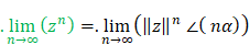
\(\lim_{n\to{\infty}}{z^n}=\ \lim_{n\to{\infty}}{\left(1+i\ \tan{\frac{\theta}{n}}\right)^n}\)
|
Eq. 88
|
Successive powers \(z^k=\ \left(1+i\tan{\frac{\theta}{n}}\right)^k\)in Eq. 88 describe a spiral that steps in \(n\) infinitesimally small increments from \(0\) to \(\theta\).
This is visualized in Figure 8 and Figure 9.
|

|
|
Figure 8: Powers of complex numbers with an infinitesimally small angle (GeoGebra)
|
|

|
|
Figure 9: Powers of complex numbers with an infinitesimally small angle (detail) (GeoGebra)
|
|
Small Angles
|
\(\frac{\theta}{n}\approx0\ \ \tan{\frac{\theta}{n}=\ }\frac{\theta}{n}\)
|
Eq. 89
|
|
|
\(\lim_{n\to{\infty}}{z^n}=\ \lim_{n\to{\infty}}{\left(1+i\frac{\theta}{n}\right)^n}\)
|
Eq. 90
|
This description is very similar to the description in "7.3.3.1 Real interpretation: "Saving".
The 'interest'\(\ \theta\ \)is divided in n steps of \(\frac{\theta}{n}\).
|
|
\(e^{i\theta}\equiv\lim_{n\to{\infty}}{\left(1+\frac{\theta}{n}i\right)^n}=\lim_{n\to{\infty}}{z^n}\)
|
Eq. 91
|
|
|
 = 1 = 1
|
Eq. 92
|
|
|

|
Eq. 93
|
|
|

|
|
|
|

\(=\lim_{n\to{\infty}}{\left(1^n\angle\left(n\arctan{\frac{\theta}{n}}\right)\right)}\)
\(=\lim_{n\to{\infty}}{\left(\ 1^n\angle\left(n\frac{\theta}{n}\right)\right)}\)
\(=1\angle\theta\)
|
Eq. 94
|
Summary:
|
|
\(e^{i\theta}\equiv{\lim_{n\to{\infty}}{\left(1+\frac{i\theta}{n}\right)^n}=\lim_{n\to{\infty}}{z^n}}\)
|
(Eq. 84)
|
|
Although we step through the angles linearly from \(0\) to \(\theta\ \)we still come to an exponential form \(e^{i\theta}\).
|
We resume Eq. 94
|
|
\(\lim_{n\to{\infty}}{\left(1^n\angle\left(n\arctan{\frac{\theta}{n}}\right)\right)}\)
\(\lim_{n\to{\infty}}{\left(\ 1^n\angle\left(n\frac{\theta}{n}\right)\right)=1\angle\theta}\)
or

|
(Eq. 94)
|
|
|
\(\cos{\left(\theta\right)}+i\sin{\left(\theta\right)}=1\angle\theta\)
|
Eq. 95
|
|
|
\(\cos{\left(\theta\right)}+i\sin{\left(\theta\right)}=1\angle\theta=\ \ {1e}^{i\theta}\)
|
Eq. 96
|
If \(k\ \)steps in infinitesimally small steps from \(0\) to \(\theta\), \({z=\left(1+i\frac{\theta}{k}\right)}^k\) describes circular arc over an angle \(\theta\), because\(z\) remains \(1\).
Extending to any arbitrary \(z\)the following is obtained:
|
|
\({re}^{i\theta}=a+bi=\ r\left(\cos{\theta}+i\sin{\theta}\right)\ \)
\(with\ r=\sqrt{a^2+b^2}\ en\ \ \theta=atan2{(b,a)}\)
|
Eq. 97
|
7.3.3.3 Euler's identity
We take the following equation from 7.3.3.2:
|
|
\({re}^{i\theta}=a+bi=\ r\left(\cos{\theta}+i\sin{\theta}\right)\ \)
\(with\ r=\sqrt{a^2+b^2}\ en\ \ \theta=atan2{(b,a)}\)
|
(Eq. 97)
|
Although we step through the angles linearly from \(0\) to \(\theta\) we still arrive at an exponential form \(e^{i\theta}\).
Substituting \(\theta=\pi\):
|
|
\({re}^{i\pi}=\ r\left(\cos{\pi}+i\sin{\pi}\right)\ \)
|
Eq. 98
|
|
Euler's Identity
|
\(1\angle\pi=\ -1+0i=\ e^{i\pi}\)
\(e^{i\pi}+1=0\)
|
Eq. 99
|
7.3.3.4 Visualization
We are now resuming Eq. 90:
|
|
\(\lim_{n\to{\infty}}{z^n}=\ \lim_{n\to{\infty}}{\left(1+\frac{\theta}{n}i\right)^n}\)
|
(Eq. 90)
|
|

|
|
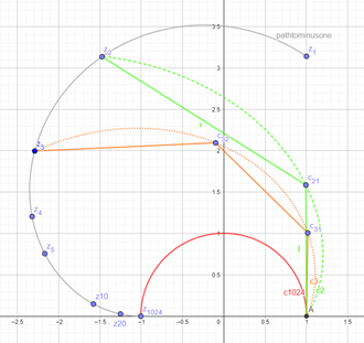
Figure 10: Path of \({z_n=\left(1+\frac{\pi}{n}i\right)}^n\)for n = 1... 1024 (GeoGebra)
|
Figure 10 shows how\(\ {z\left(n\right)=z_n=\left(1+\frac{\pi}{n}i\right)}^n\)evolves to-1 as \(n\in\mathbb{N}\ \)increases.
The curve 'Pathtominusone' arises when\(\ z\left(v\right)=\left(1+\frac{\pi}{v}i\right)^v,v\ \in\mathbb{R}\ \)is drawn.
To exactly represent the reasoning, only the discrete points \(z_n\)should have been shown.
Figure 11 shows how \({c_n\left(k\right)=\left(1+\frac{\pi}{n}i\right)}^kwith\ k,\ n\in\mathbb{N}\) approximates a semi-circle better as \(n\ \)increases.
The end point of is \(z_n{=c}_n\left(n\right).\)the 'angle of the point \(z_n\)'\(=n\ \ \arctan{\frac{\pi}{n}}\)
|
|
|
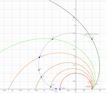
Figure 11: Half-circle approximated by \(c_n\left(k\right)=\left(1+\frac{\pi}{n}i\right)^k\)for n = 2.3 and 1024 (GeoGebra)
|
As \(k\ \)runs from \(0\) to \(n\), \({c_n(k)=\lim_{n\to{\infty}}\left(1+\frac{\pi}{n}i\right)}^kwith\ k,n\ \in\mathbb{N}\ \)describes a semi-circle, because\(z\)remains \(1\).
If the discrete parameter \(k\ \in\mathbb{N}\) is replaced by\(\ v\in\mathbb{R}\)
\({c_n(v)=\lim_{n\to{\infty}}\left(1+\frac{\pi}{n}i\right)}^vwith\ v\ \in\mathbb{R}\ ,n\ \in\mathbb{N}\ \)describes a spiral approximating the unit circle more and more.
This is visualized in Figure 12.
|
|
|
Figure 12: semi-circle approximated by \(c_n\left(v\right)=\left(1+\frac{\pi}{n}i\right)^v\)for n = 1, 2, 3, 5, 10, 1024 (GeoGebra)
|
The spirals are extended to the negative x-axis.
7.3.3.5 Starting from De Moivre
The following derivation is literally taken from (iLearn - Complexe getallen : formule van Euler, sd)
|
Can we reformulate the formula of De Moivre so a definition or feature of it \(e^x\)can be applied?
|
|
De Moivre
|
\(\left(\cos{\alpha}+i\sin{\alpha}\right)^n=\ 1^n\angle\left(n\alpha\right)=\cos{\left(n\alpha\right)}+i\sin{\left(n\alpha\right)}\)
|
(Eq. 1)
|
Substitute \(\alpha=\frac{\theta}{n}\)
|
|
\(\cos{\left(n\frac{\theta}{n}\right)}+i\sin{\left(n\frac{\theta}{n}\right)}=\ \left(\cos{\left(\frac{\theta}{n}\right)}+i\sin{\left(\frac{\theta}{n}\right)}\right)^n\)
|
Eq. 100
|
Simplify \(n\frac{\theta}{n}=\ \theta\)
|
|
\(\cos{\theta}+i\sin{\theta}=\left(\cos{\frac{\theta}{n}}+i\sin{\frac{\theta}{n}}\right)^n\)
|
Eq. 101
|
Apply the limit:
|
|
\(\lim_{n\to{\infty}}{\left(\cos{\theta}+i\sin{\theta}\right)}=\ \lim_{n\to{\infty}}{\left(\cos{\left(\frac{\theta}{n}\right)}+i\sin{\left(\frac{\theta}{n}\right)}\right)^n}\)
|
Eq. 102
|
|
Small Angles
|
\(\frac{\theta}{n}\ \approx0\ \Rightarrow\ \cos{\left(\frac{\theta}{n}\right)}\approx1\ en\ \sin{\frac{\theta}{n}}\approx\frac{\theta}{n}\)
|
Eq. 103
|
|
|
\(\lim_{n\to{\infty}}{\left(\cos{\theta}+i\sin{\theta}\right)}=\lim_{n\to{\infty}}{\left(1+i\ \left(\frac{\theta}{n}\right)\right)^n}\)
|
Eq. 104
|
|
Final
|
\(e^x\equiv\lim_{n\to{\infty}}{\left(1+\frac{x}{n}\right)^n}\)
|
(Eq. 83)
|
Substitute \(x=i\theta\)
|
|
\(\left(\cos{\theta}+i\sin{\theta}\right)=\ \lim_{n\to{\infty}}{\left(1+i\ \frac{\theta}{n}\right)^n=\ e^{i\theta}}\)
|
Eq. 105
|
8 References
Wikipedia - Complex Number. (n.d.). Retrieved from Wikipedia: https://en.wikipedia.org/wiki/Complex_number
Bombelli, R. (1572). L'ALGEBRA. Bologna.
iLearn - Complexe getallen : formule van Euler. (n.d.). Retrieved from iLearn: https://youtu.be/pD_nxOtJ_FQ
math.as.uky.edu/ Part 2: Cardano’s Ars Magna. (n.d.). Retrieved from College of Arts & Sciences: http://www.ms.uky.edu/~sohum/ma330/files/eqns_2.pdf
Merino, O. (2006). A Short History of Complex Numbers. University of Rhode Island.
The RC Filter Transfer Function. (2015, 12 15). Retrieved from Analog Zoo: http://www.analogzoo.com/2015/12/deriving-the-rc-filter-transfer-function/
uhasselt@school - Lesmateriaal - Complexe getallen. (n.d.). Retrieved from uhasselt.be: https://www.uhasselt.be/documents/uhasselt@school/lesmateriaal/wiskunde/matcom/Lesmateriaal/Comp.pdf
Wagner, R. (2009). The geometry of the unknown: Bombelli’s algebra linearia. Philosophical Aspects of Symbolic Reasoning in Early Modern Science and Mathematics (PASR). Gent: UGent.
Wikipedia - atan2. (n.d.). Retrieved from Wikipedia: https://en.wikipedia.org/wiki/Atan2
Wikipedia - De Moivre's formula. (n.d.). Retrieved from Wikipedia: https://en.wikipedia.org/wiki/De_Moivre%27s_formula
Wikipedia - Euler's formula. (n.d.). Retrieved from Wikipedia: https://en.wikipedia.org/wiki/Euler%27s_formula
Wikipedia - Exponential function. (n.d.). Retrieved from Wikipedia: https://en.wikipedia.org/wiki/Exponential_function
Wikipedia - Oliver Heaviside. (n.d.). Retrieved from Wikipedia: https://en.wikipedia.org/wiki/Oliver_Heaviside
Wikiquote - Euler's identity. (n.d.). Retrieved from Wikiquote: https://en.wikiquote.org/wiki/Euler%27s_identity