1 Goal

This document aims to construct the essential elements of linear algebra applied to linear transformations in an intuitive way,
starting from real-world problems or concrete questions.

The document starts with elementary linear transformations and builds incrementally until the singular-value decomposition emerges after a rare leap-of-faith.

The starting point of the document is the belief the best approach to mathematics for many students is starting from questions and problems
in physical reality.

Sometimes the examples in the document may be somewhat artificial.
Their added value is that they allow the reader to connect real-world situations or visual representations with mathematical concepts.

Once the student has acquired a feeling of mastery, the knowledge can be embedded in a clean, correct, and complete mathematical framework of structures,
theorems, and properties.

Using the analogy with language teaching, sentence analysis is not first formally taught and then applied.
A child learns and uses language and only when the mastery is sufficient, sentences are formally analyzed.

Until the twentieth century, most of the mathematics was firmly founded in reality, developed to solve real-world-problems.
Only in the twentieth century have mathematicians come to invent mathematical concepts and structures that are entirely isolated from physical reality.

All the giants of mathematics until the twentieth century were mainly concerned with physical problems.

2 Prerequisites

To read and digest this document a basic understanding of coordinate systems, basis and basis-changes, vector-calculation and
matrix-calculation is required.

3 Introduction

Nothing in mathematics is trivial.

The mathematics taught to high-school students nowadays has evolved over more than two thousand years.
What is taught to teens today was the most complex mathematics twenty centuries ago.

A Babylonian tablet from about 300 BC states the following mathematical problem.
Solving that problem was science:

There are two fields whose total area is 1800 square yards. One produces grain at the rate of 2/3 of a bushel per square yard
while the other produces grain at the rate of 1/2 a bushel per square yard. If the total yield is 1100 bushels, what is the size of each field?
(MacTutor - Matrices and determinants, sd)

In today’s notation, the formalization of the problem looks as shown below:

\(\frac{bushels}{sq\ yard}sq\ yard\ +\frac{bushels}{sq\ yard}sq\ yard\ =\frac{2}{3}x+\ \frac{1}{2}y=1100=bushels\)

\(sq\ yard\ +sq\ yard\ =1x+\ 1y=1800=\ sq\ yard\)

In 1303 AD, the Chinese mathematician Zhu Shijie used a notation resembling a matrix, and he described a procedure much alike Gaussian elimination to solve systems of linear equations. (Wikipedia - Zhu Shijie, sd)

Matrix-calculus was only formalized in 1858 by Cayley. He defined the concept ‘matrix’, the elementary operations, and some properties.

Before him, giants like Leibniz (1710), Laplace (1772), Lagrange (1773), Gauss (1801), Cauchy (1826) had made steps towards matrix-calculus.

Leibniz came very close in 1693 but got stuck close to the real ‘aha-erlebnis’.

Leibniz: \(ij\)	‘now’: \(a_{ij}\)
\(10+11\ x+12\ y=0\) \(20+21\ x+22\ y=0\) \(30+31\ x+32\ y=0\)	\(-b_1+\ a_{12}x+\ a_{13}y=0\) \({-b}_2+\ a_{22}x+\ a_{23}y=0\) \(-b_3+\ a_{32}x+\ a_{33}y=0\)
	\(a_{11}x+\ a_{12}y=b_1\) \(a_{21}x+\ a_{22}y=b_2\) \(a_{31}x+\ a_{32}y=b_3\)
	\(\left[\begin{matrix}a_{11}&a_{12}\\a_{21}&a_{22}\\a_{31}&a_{32}\\\end{matrix}\right]\left[\begin{matrix}x\\y\\\end{matrix}\right]=\left[\begin{matrix}b_1\\b_2\\b_3\\\end{matrix}\right]\)

All those giants had one enormous advantage compared to today’s students: they started from real-life problems.
Most often they had a solution in mind, but they were struggling to find a practical notation, a language to formalize their thinking or write down their solution strategy.

This document only covers linear transformations on the plane, represented with simple-to-handle 2x2-matrices and operations that can be visualized in the two dimensions of a sheet or a screen.

As said, the examples and ‘triggering questions’ may be artificial, but their only intention is to connect mathematics with reality or
the imagination of the reader.

The document does not have the ambition to be complete, but it has the ambition to be correct.

3.1 What is being transformed?

The relationship between mathematical operations and reality can be constructed in many different ways.
The ‘user of mathematics’ can freely determine how that relationship is constructed, as long as it contributes to describing and solving the problem at hand.

3.1.1 Photoshopping

Later in the document, some examples will be used where operations are described on objects on a screen, vector-drawings, and photos or bitmaps. When a photo is being transformed, each pixel has to be moved on the screen:

A picture is:

· rotated,

· sheared,

· scaled or,

· moved on the screen, translated.

The term shearing is used because the effect resembles cutting the picture in strips that shift like a landslide.
The transformation also corresponds to a deformation called ‘shear’ in material science.

transformations on a picture or bitmap

Fig. 1: transformations on a picture or bitmap

3.1.2 Movement of an object on a plane

Suppose the movement of an object is to be described, where only the position and not the orientation of the object of interest.

In such situations, all calculations are made for one point of the body.

If the mass of the object is necessary, the mass center of the object will probably be chosen.

If the object's orientation is essential, it is required to describe the movement of at least two points of the object.
Often the movement is then split into two components: the movement of the mass center and the rotation of the object around the mass center.

In the figure below, it is chosen to describe the movement of one vertex of the car:

transformations on a picture or bitmap

Fig. 2: transformations on a picture or bitmap

4 Conventions

4.1 Free vectors, sliding, bound vectors, and location

Depending on the application, free, sliding, or bound vectors are used.

If you want to describe that a vector expresses the same regardless of where it is located on the plane, the vector is called ' free '.
You are free to put the vector where you want.

A free vector defines a direction and a length.

If you want to describe that a vector expresses the same, regardless of where it is located on a line, it is called a sliding vector.
You can slide the vector over the straight line. The vector expresses the same everywhere.

A sliding vector determines a line and a length.

A bound vector is attached to a starting point or initial point.
A bound vector thus determines two points and a sequence of those two points or an initial point, a direction, and a length.

A special kind of bound vectors are the position vectors. A position or location vector has the origin as its initial point.
Therefore, a place vector defines one point, one location, the endpoint of the vector.

Further, in this document, space vectors are used, unless the contrary is explicitly stated.
When using location vectors, the notations of a point and a vector are interchangeable:

The vector \(\vec{op}\) is a location vector, \(\vec{op}\) is equivalent to \(\vec{p}\).
\(\vec{p}\) has coordinates \(\left[\begin{matrix}p_x\\p_y\\\end{matrix}\right]_{uv}or\ \left(p_x,p_y\right)\ or\ p\left(p_x,p_y\right)\)

\(\vec{p}=\) \(\left(p_x,p_y\right)=p=\ \vec{op}\ \ \Longleftrightarrow\ \vec{p}\ is\ a\ \ location\ vector\)

4.2 Transformations and matrices

In the MS Word version of this document, transformations are indicated with a script letter
In the web version, transformations are indicated with a \(\mathfrak{fraktur}\ \mathfrak{letter}\) corresponding to LateX “\ mathfrak”
because LateX “\ mathcal” small letters do not show as script letters. I hope Hilbert can forgive me for doing so.
Matrices are denoted using CAPITALS.
Angles are indicated with a Greek letter.

Operation	Matrix	Transformation	Components
<T>ranslation by \(t_x,\ t_y\)	\(T\)	\(\mathfrak{t}\)	\(t_x,\ t_y\)
<R>otation over an angle α	\(R\ or\ R_\alpha\ or\ R\left(\alpha\right)\)	\(\mathfrak{r}\ or\ \mathfrak{r}_{\alpha\ }or\ \mathfrak{r}\left(\alpha\right)\)	α
<S>caling by s	\(S\ or\ S_s\ or\ S\left(s\right)\)	\(\mathfrak{s}\ or\ \mathfrak{s}_s\ or\ \mathfrak{s}\left(s\right)\)	\(s\ or\ s_x,s_x\)

4.3 Transformations and change of basis

When studying change of basis one gets easily lost, confused in terms of which basis a vector is being expressed.

Therefore a vector can be suffixed with the name of the basis:
Vector \(\vec{p}\) has coordinates \(\left[\begin{matrix}p_x\\p_y\\\end{matrix}\right]_{uv}\ of\ \left(p_x,p_y\right)_{uv}\)expressed in terms of basis \(\left\{\vec{u},\ \vec{v}\right\}\).

To discriminate between a transformation and a change of basis, a change of basis is indicated with script letter \(\mathfrak{b}\) ,
so a change of basis is denoted as: \({\vec{u}}_{kl}\buildrel\mathfrak{b}\over\rightarrow{\vec{u}}_{uv}\).

4.4 Cartesian and polar coordinates

When there is a risk of confusion between polar and Cartesian coordinates a suffix \(polar\) of \(cart\) is used:

\({p\left(p_x,p_y\right)}_{cart}={p\left(r\ \cos{\theta},r\ \sin{\theta}\right)}_{cart}={p\left(r\ ,\theta\right)}_{polar}\)

\(where\ r=\sqrt{{p_x}^2+{p_y}^2}and\ \theta=atan2\left(p_y,p_x\right)\)

4.5 Angles

Angles are indicated with \(\angle\) or a \(\widehat{hat}\).

\(\theta=\angle\left(\vec{a},\vec{b}\right)=\widehat{\vec{a},\vec{b}}\)

4.6 Changing or transforming & mapping

To avoid confusion between transformations and change of basis, the verbs ‘changing’ or ‘converting’ is used when changing basis.
For a transformation, the verbs ‘transforming’ or ‘mapping’ are used.

When changes of basis are described, the original basis is typically denoted as \(\left\{\vec{k}\right\},\ \left\{\vec{k},\ \vec{l}\right\}\)and the new basis is \(\left\{\vec{u}\right\},\ \left\{\vec{u},\ \vec{v}\right\}\ \).

The changes of basis from \(\left\{\vec{k},\ \vec{l}\right\}\) to \(\left\{\vec{u},\ \vec{v}\right\}\) changes the coordinates of the vector \(\vec{p}\) from \(\left[\begin{matrix}3\\1\\\end{matrix}\right]_{kl}\)to \(\left[\begin{matrix}-1\\-1\\\end{matrix}\right]_{uv}.\)

change of basis

Fig. 3: change of basis

The point \(\vec{p}\) does not move, but the reference frame, the basis, changes.

The car stays where it is, but we describe its position in terms of a new frame of reference.

The linear transformation \(\mathfrak{t}\) transforms the vector \(\vec{p}\) with coordinates \(\left[\begin{matrix}p_x\\p_y\\\end{matrix}\right]_{kl}\) to \(\vec{q}\) having coordinates \(\left[\begin{matrix}q_x\\q_y\\\end{matrix}\right]_{kl}\).

\(\vec{p}\)=\(\left[\begin{matrix}p_x\\p_y\\\end{matrix}\right]_{kl}{\buildrel\mathfrak{t}\over\rightarrow}\vec{q}\)=\(\left[\begin{matrix}q_x\\q_y\\\end{matrix}\right]_{kl}\).

transformation

Fig. 4: transformation

The reference frame \(\left\{\vec{k},\ \vec{l}\right\}\ \)remains the same, but the point \(\vec{p}\) is mapped onto the point \(\vec{q}.\)

The car is moved from \(\vec{p}\) to \(\vec{q}\).

4.7 Frame of Reference

Reasoning about changes of basis and transformations can be confusing.
When \(\vec{p}\) is a point of an object, a car, a transformation moves the car. If it is a real car, the car moves. I am in a car, and I experience a movement.

When we consider a change of basis, all of the universe stays where it is, but the frame of reference in terms of which we express positions
is changed.

If I move the origin of my coordinate system from Brussels to Amsterdam, I do not move, but my coordinates change.

The changes of basis in this document preserve the location of the origin, but they change orientation, and the reference-length used to express distances and lengths.
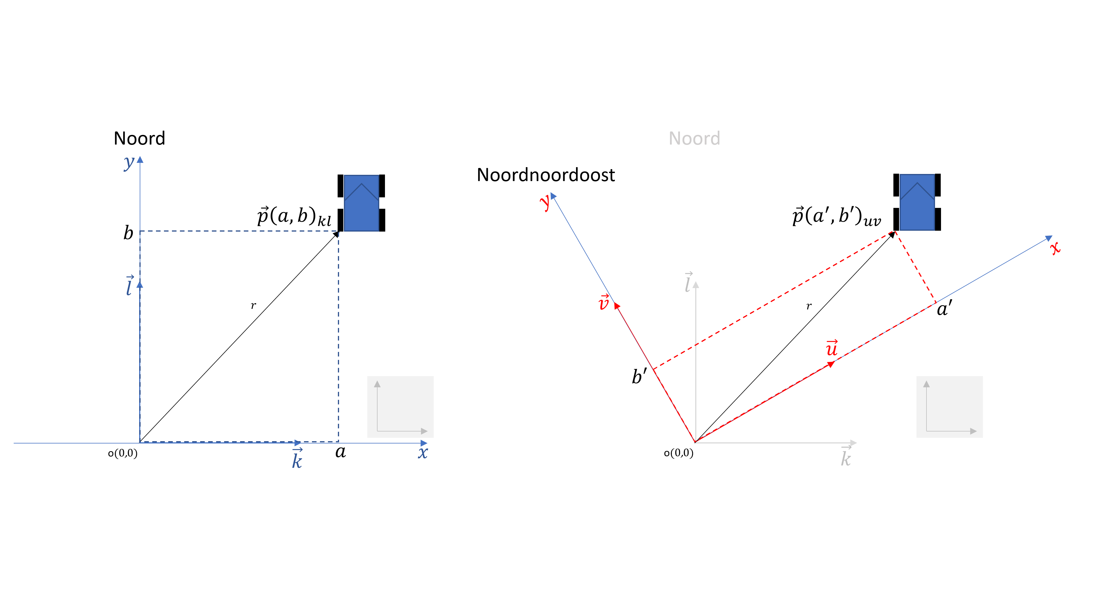
Considering Fig. 6, suppose we start with a basis \(\left\{\vec{k},\ \vec{l}\right\}\) in which the basis-vector \(\vec{l}\ \)points North, then \(\vec{v}\) of the basis \(\ \left\{\vec{u},\ \vec{v}\right\}\) points North-Northwest.
Suppose I am at \(\vec{p}\), then I do not move, but my coordinates change.

To keep clear what is being changed, this document adds a third ‘absolute’ coordinate system in all figures describing changes of basis.
This coordinate system has a fixed position and orientation.

'absolute' frame of reference

Fig. 5: 'absolute' frame of reference

In this document, this coordinate system can be considered ‘absolute’.

change of basis and third basis as reference

Fig. 6: change of basis and third basis as reference

4.8 Abstract transformations

Transformations are often used to describe ‘state changes’ in a system. Rather than a location of an object, physical quantities are described
(volume pressure, voltage). The described system moves in an abstract ‘state space’.

Fig. 7 shows a state change of a cylinder and valve described in the (V,P)-plane.

The valve moves up, the volume increases and the pressure decreases.

transformation in (V,P)-plane

Fig. 7: transformation in (V,P)-plane

4.9 Mysterious dots

Some of the expressions in this document are preceded by a ‘.’, a dot, this has no semantics for the human reader.
It only indicates that the MSWord does not produce correct LateX for these expressions, so they are converted into bitmaps when creating a web version.

5 Transformation

5.1 Operations

When an object in a computer game moves over the screen, the object is moved by redrawing it over and over by applying transformations on each individual pixel of the object.

When the movement of an object in a plane is described, often the position of one single point of the object is calculated, often the center of mass.

Each elementary movement can be described as a transformation. Sometimes the object moves over an infinitesimally small step \((dx,dy,dz)\) ,
sometimes it moves over a finite step \((\mathrm{\Delta\ x},\mathrm{\Delta\ y},\mathrm{\Delta\ z})\).

Transformations are constructed from three elementary transformations:

1. A Translation

2. A Rotation

3. A Scaling

A translation is not a linear transformation: linear transformations preserve the origin, they map the origin onto itself.

5.2 Translation

When a car drives along a straight line over the screen, the graphics card will calculate the position of the car multiple times per second and
shift the bitmap of the car from its old to its new position.
If the positions are calculated very often, the steps \(\left(t_x,t_y\right)\) are small and the car will move smoothly. If not the car will jump from position to position.

car drives along a straight line

Fig. 8: car drives along a straight line

An object to be displayed on a computer screen is described as a bitmap or a vector drawing.

5.2.1 Moving a vector-drawing

A vector drawing is stored as a series of points. When a vector drawing is displayed, the computer draws line segments or vectors between the consecutive points.

When the last point connects to the first point, the series describes a polygon.

If a vector drawing is moved, the new positions of all points must be calculated and the points must be connected by segments.

In computer-graphics the points of a vector drawing are called vertices, even if the series is not closed to be a polygon.
The term vertex is then used to discriminate it from an isolated point.

Triangle is being translated

Fig. 9: Triangle is being translated

\({triangle}_1\)

\(=\left\{\left(x_{a1},y_{a1}\right),\left(x_{b1},y_{b1}\right),\left(x_{c1},y_{c1}\right)\right\}\)

\(=\mathfrak{t}\left({triangle}_0\right)\)

\(=\left\{\mathfrak{t}\left(\left(x_{a0},y_{a0}\right)\right),\mathfrak{t}\left(\left(x_{b0},y_{b0}\right)\right),\mathfrak{t}\left(\left(x_{c0},y_{c0}\right)\right)\right\}\)

\(=\left\{\left(x_{a0}+t_x,y_{a0}+t_y\right),\left(x_{b0}+t_x,y_{b0}+t_y\right),\left(x_{c0}+t_x,y_{c0}+t_y\right)\right\}\)

5.2.2 Moving a bitmap

A picture is stored in a computer as a bitmap.

When a picture is moved over the screen, a new position for each pixel is to be calculated.

To move the picture in Fig. 10 all 13x18=234 pixels must be moved.

picture of a person in a 13x18 pixel resolution

Fig. 10: picture of a person in a 13x18 pixel resolution

translation of a picture

Fig. 11: translation of a picture

\({photo}_1\)

\(=\left\{\left(x_{k1},y_{l1}\right)|k\in\left[0\ldots12\right],l\in\left[0\ldots17\right]\right\}\)

\(=\mathfrak{t}\left({photo}_0\right)\)

\(=\left\{\mathfrak{t}\left(\left(x_{k0},y_{l0}\right)\right)|k\in\left[0\ldots12\right],l\in\left[0\ldots17\right]\right\}\)

\(=\left\{\left(x_{k0}+t_x,y_{l0}+t_y,kleur\right))|k\in\left[0\ldots12\right],l\in\left[0\ldots17\right]\right\}\)

5.2.3 Translation as a matrix

Can the operation \(\left(x_0,y_0\right)\ {\buildrel\mathfrak{t}\over\rightarrow\ }\left(x_1,y_1\right)=\left(x_0+t_x,y_0+t_y\right)\) be written as a matrix operation?

Can a translation be written as a matrix-product?

\(X_1=TX_0\)

We rewrite the translation, trying to make it resemble a product of matrices:

	\(x_1=x_0+t_x\)
	\(x_1=1\ x_0+0{\ y}_0+{\ t}_x1\)	Exp. 1

	\(y_1=y_0+t_y\)
	\(y_1=0{\ x}_0+1\ y_0+{\ t}_y1\)	Exp. 2

Exp. 2 is now written as a product of matrices:

\(\left[\begin{matrix}x_1\\y_1\\1\\\end{matrix}\right]=\left[\begin{matrix}1&0&{\ t}_x\\0&1&{\ t}_y\\0&0&1\\\end{matrix}\right]\left[\begin{matrix}x_0\\y_0\\1\\\end{matrix}\right]=T\left[\begin{matrix}x_0\\y_0\\1\\\end{matrix}\right]\)

Exp. 3

Is it possible to write \(\ {\left(x_1,y_1\right)\buildrel\mathfrak{t}^{-1}\over\rightarrow\ \left(x_0,y_0\right)}=\left(x_1-t_x,y_1-t_y\right)\) as a product of matrices?

\(\left[\begin{matrix}x_0\\y_0\\1\\\end{matrix}\right]=\left[\begin{matrix}1&0&{-t}_x\\0&1&{-\ t}_y\\0&0&1\\\end{matrix}\right]\left[\begin{matrix}x_1\\y_1\\1\\\end{matrix}\right]\)

Exp. 4

Is the 3x3 matrix in Exp. 4 the inverse matrix of the 3x3 matrix \(T\) in Exp. 3?

\(\left[\begin{matrix}1&0&{-t}_x\\0&1&{-\ t}_y\\0&0&1\\\end{matrix}\right]T=\left[\begin{matrix}1&0&{-t}_x\\0&1&{-\ t}_y\\0&0&1\\\end{matrix}\right]\left[\begin{matrix}1&0&{\ t}_x\\0&1&{\ t}_y\\0&0&1\\\end{matrix}\right]=\left[\begin{matrix}1&0&0\\0&1&0\\0&0&1\\\end{matrix}\right]\)

Exp. 5

We try it out and, yes!

\(T=\left[\begin{matrix}1&0&{\ t}_x\\0&1&{\ t}_y\\0&0&1\\\end{matrix}\right]en\ \left[\begin{matrix}1&0&{-t}_x\\0&1&{-\ t}_y\\0&0&1\\\end{matrix}\right]=T^{-1}\)

Exp. 6

5.2.4 Translation combined with other operations

We resume Exp. 1 and Exp. 2:

	\(x_1=1\ x_0+0{\ y}_0+{\ t}_x1\)	(Exp. 1)
	\(y_1=0{\ x}_0+1\ y_0+{\ t}_y1\)	(Exp. 2)

	\(x_1=a_{11}{\ x}_0+a_{21}{\ y}_0+{\ t}_x1\)	Exp. 7
	\(y_1=a_{21}\ x_0+{a\ }_{22}y_0+{\ t}_y1\)	Exp. 8

	\(\left[\begin{matrix}x_1\\y_1\\\end{matrix}\right]=\left[\begin{matrix}a_{11}&a_{12}\\a_{21}&a_{22}\\\end{matrix}\right]\left[\begin{matrix}x_0\\y_0\\\end{matrix}\right]+\left[\begin{matrix}t_x\\t_y\\\end{matrix}\right]\)	Exp. 9
	\(\left[\begin{matrix}x_1\\y_1\\\end{matrix}\right]=A\left[\begin{matrix}x_0\\y_0\\\end{matrix}\right]+\left[\begin{matrix}t_x\\t_y\\\end{matrix}\right]\ with\ A=\left[\begin{matrix}a_{11}&a_{12}\\a_{21}&a_{22}\\\end{matrix}\right]\)	Exp. 10

\(\left[\begin{matrix}x_1\\y_1\\1\\\end{matrix}\right]=\left[\begin{matrix}a_{11}&a_{12}&{\ t}_x\\a_{21}&a_{22}&{\ t}_y\\0&0&1\\\end{matrix}\right]\left[\begin{matrix}x_0\\y_0\\1\\\end{matrix}\right]=T\left[\begin{matrix}x_0\\y_0\\1\\\end{matrix}\right]\)

Exp. 11

Exp. 12

We conclude that the translation can be combined with operations of the form:

\(\left[\begin{matrix}x_1\\y_1\\\end{matrix}\right]=\left[\begin{matrix}a_{11}&a_{12}\\a_{21}&a_{22}\\\end{matrix}\right]\left[\begin{matrix}x_0\\y_0\\\end{matrix}\right]\ of\ \left[\begin{matrix}x_1\\y_1\\\end{matrix}\right]=A\left[\begin{matrix}x_0\\y_0\\\end{matrix}\right]\ with\ A=\left[\begin{matrix}a_{11}&a_{12}\\a_{21}&a_{22}\\\end{matrix}\right]\)

Exp. 13

5.3 Rotation

Can we write the rotation of a point or location vector as a matrix-product?

(Inverse) rotation of a photo

Fig. 12: (Inverse) rotation of a photo

5.3.1 Rotation of a point

If we rotate a vector, its length does not change, only the angle relative to the axes.
Let us rotate the point \(a_0\ \)over an angle \(\alpha\) around the origin \(o\) to the point \(a_1\).

rotation of a point

Fig. 13: rotation of a point

Every point or vector \(a\left(x_{a0},y_{a0}\right)\) can be written as \(\left(r.\cos{\theta},r.\sin{\theta}\right):\)

\(a\left(x_{a0},y_{a0}\right)=a\left(r.\cos{\theta},r.\sin{\theta}\right)\)

\(with\ r=\sqrt{{x_{a0}}^2+{y_{a0}}^2}\ and\ \theta=atan2{\left(y_{a0}{,x}_{a0}\right)}\)

Exp. 14

\(\mathfrak{r}_\alpha\left(\left(x_{a0},y_{a0}\right)\right)\)

\(=\mathfrak{r}_\alpha\left(\left(r.\cos{\theta},r.\sin{\theta}\right)\right)\)

Exp. 15

If we rotate the vector with angle \(\theta\) relative tot the x-axis over an angle \(\alpha\), the result is a vector with the same length, and angle \(\theta+\alpha:\)

	\(\left(x_{a1},y_{a1}\right)\)	\(=\left(r.\cos{\left(\theta+\alpha\right)},r.\sin{\left(\theta+\alpha\right)}\right)\)
		\(=r\left(\cos{\left(\theta+\alpha\right)},\sin{\left(\theta+\alpha\right)}\right)\)	Exp. 16

We apply the following identities to Exp. 16:

	\(\cos{\left(\theta+\alpha\right)}=\cos{\theta}\cos{\alpha}-\sin{\theta}\sin{\alpha}\)	Exp. 17
	\(\sin{\left(\theta+\alpha\right)}=\sin{\theta}\cos{\alpha}+\cos{\theta}\sin{\alpha}\)	Exp. 18

\(\mathfrak{r}_\alpha\left(\left(x_{a0},y_{a0}\right)\right)=r\left(\cos{\left(\theta+\alpha\right)},\sin{\left(\theta+\alpha\right)}\right)\)

(Exp. 16)

\(x_{a1}=r\left(\cos{\theta}\cos{\alpha}-\sin{\theta}\sin{\alpha}\right)\)

\(y_{a1}=r\left(\sin{\theta}\cos{\alpha}+\cos{\theta}\sin{\alpha}\right)\)

Exp. 19

\(x_{a1}=\left(r\cos{\theta}\cos{\alpha}-r\sin{\theta}\sin{\alpha}\right)\)

\(y_{a1}=\left(r\sin{\theta}\cos{\alpha}+r\cos{\theta}\sin{\alpha}\right)\)

Exp. 20

\(x_{a1}=\left(\cos{\alpha}r\cos{\theta}-\sin{\alpha\ r\sin{\theta}}\right)\)

\(y_{a1}=\left(\sin{\alpha}r\cos{\theta}+\cos{\alpha}r\sin{\theta}\right)\)

Exp. 21

\(x_{a1}=\left(\cos{\alpha}x_{a0}-\sin{\alpha}{\ y}_{a0}\right)\)

\(y_{a1}=\left(\sin{\alpha}x_{a0}+\cos{\alpha}\ y_{a0}\right)\)

Exp. 23

Rotating a vector \(a\left(x_{a0},y_{a0}\right)\) over an angle \(\alpha\) can be expressed as a matrix multiplication

\(\left[\begin{matrix}x_{a1}\\y_{a1}\\\end{matrix}\right]=\left[\begin{matrix}\cos{\alpha}&-\sin{\alpha}\\\sin{\alpha}&\cos{\alpha}\\\end{matrix}\right]\left[\begin{matrix}x_{a0}\\x_{a0}\\\end{matrix}\right]\)

Exp. 24

If the angle of \(a\left(x_{a0},y_{a0}\right)\) was \(\theta\), then the new angle is \(\theta+\alpha\).

5.3.2 Rotation of a point on an axis

Does considering the rotation of a point on a coordinate axis bring better insight into the nature of a rotation matrix?

First, the rotation of ‘any’ vector on an axis is considered, later we consider the rotation of a unit vector on an axis.

5.3.2.1 Rotation of a point on the x-axis

The point \(a_0\) has coordinates \(\left(r,0\right)\) in terms of the orthonormal basis \(\left\{\vec{k},\vec{l}\right\}.\)
We look for the coordinates of \(a_1\), the result of rotating \(a_0\) over an angle \(\alpha.\)
The coordinates of \(a_1\) is expressed in terms of the orthonormal basis \(\left\{\vec{k},\vec{l}\right\}.\)

rotation of a point on the x-axis

Fig. 14: rotation of a point on the x-axis

Every point \(\left(x_{a0},y_{a0}\right)\ \)on the x-axis can be written as \(\left(r,0\right).\)

\(a_0\left(x_{a0},y_{a0}\right)\)

\(=a_0\left(r,0\right)\ =\ \left(r.\cos{\left(0\right)},r.\sin{\left(0\right)}\right)\)

Exp. 25

When the vector on the x-axis is being rotated over an angle \(\alpha\), the length is preserved but the angle changes:

\(\mathfrak{r}_\alpha\left(\left(x_{a0},y_{a0}\right)\right)\)	\(=\mathfrak{r}_\alpha\left(\left(r,0\right)\right)\)	Exp. 26
	\(=\left(r.\cos{\left(\alpha\right)},r.\sin{\left(\alpha\right)}\right)\)
	\(=r\left(\cos{\left(\alpha\right)},\sin{\left(\alpha\right)}\right)\)	Exp. 27

In general, a rotation over an angle \(\alpha\) can be expressed as a matrix multiplication:

(Exp. 24)

We apply Exp. 24 to \(a_0\left(x_{a0},y_{a0}\right)=\left(r,0\right)=\ \left[\begin{matrix}r\\0\\\end{matrix}\right]:\)

\(\left[\begin{matrix}x_{a1}\\y_{a1}\\\end{matrix}\right]=\left[\begin{matrix}\cos{\alpha}&-\sin{\alpha}\\\sin{\alpha}&\cos{\alpha}\\\end{matrix}\right]\left[\begin{matrix}r\\0\\\end{matrix}\right]\)

Exp. 28

\(\left[\begin{matrix}x_{b1}\\y_{b1}\\\end{matrix}\right]=\left[\begin{matrix}\cos{\alpha}r-\sin{\alpha\ 0}\\\sin{\alpha}r+\cos{\alpha}0\\\end{matrix}\right]\)

Exp. 29

\(\left[\begin{matrix}x_{b1}\\y_{b1}\\\end{matrix}\right]=\left[\begin{matrix}\cos{\alpha}r-\sin{\alpha\ 0}\\\sin{\alpha}r+\cos{\alpha}0\\\end{matrix}\right]\)

Exp. 30

\(\mathfrak{r}_\alpha\left(\left[\begin{matrix}r\\0\\\end{matrix}\right]\right)=\left[\begin{matrix}x_{b1}\\y_{b1}\\\end{matrix}\right]=r\left[\begin{matrix}\cos{\alpha}\\\sin{\alpha}\\\end{matrix}\right]\)

Exp. 31

When a vector with length \(r\) on the x-axis is rotated over an angle \(\alpha\), the result is the first column of the corresponding rotation-matrix, multiplied by \(r\).

5.3.2.2 Rotation of a point on the y-axis

The point \(b_0\) has coordinates \(\left(0,r\right)\) expressed in terms of the orthonormal basis \(\left\{\vec{k},\vec{l}\right\}.\)
We look for the coordinates of the point \(b_1\), the result of rotating \(a_1\) over an angle \(\alpha.\)
The coordinates of \(a_1\) are expressed in terms of the orthonormal basis \(\left\{\vec{k},\vec{l}\right\}.\)

rotation of a point on the y-as

Fig. 15: rotation of a point on the y-as

\(b\left(x_{b0},y_{b0}\right)\)

\(=b\left(0,r\right)\ \)

Exp. 32

\(\mathfrak{r}_\alpha\left(\left(x_{b0},y_{b0}\right)\right)\)	\(=\mathfrak{r}_\alpha\left(\left(0,r\right)\right)\)	Exp. 33
	\(=\left(-r.\sin{\left(\alpha\right)},r.\cos{\left(\alpha\right)}\right)\)
	\(=r\left(-\sin{\left(\alpha\right)},\cos{\left(\alpha\right)}\right)\)	Exp. 34

	\(\left[\begin{matrix}x_{b1}\\y_{b1}\\\end{matrix}\right]=\left[\begin{matrix}\cos{\alpha}&-\sin{\alpha}\\\sin{\alpha}&\cos{\alpha}\\\end{matrix}\right]\left[\begin{matrix}0\\r\\\end{matrix}\right]\)	Exp. 35
	\(\left[\begin{matrix}x_{b1}\\y_{b1}\\\end{matrix}\right]=\left[\begin{matrix}\cos{\alpha}0-\sin{\alpha\ r}\\\sin{\alpha}0+\cos{\alpha}r\\\end{matrix}\right]\)	Exp. 36
	\(\left[\begin{matrix}x_{b1}\\y_{b1}\\\end{matrix}\right]=\left[\begin{matrix}\cos{\alpha}0-\sin{\alpha\ r}\\\sin{\alpha}0+\cos{\alpha}r\\\end{matrix}\right]\)	Exp. 37

\(\mathfrak{r}_\alpha\left(\left[\begin{matrix}0\\r\\\end{matrix}\right]\right)=\left[\begin{matrix}x_{b1}\\y_{b1}\\\end{matrix}\right]=r\left[\begin{matrix}-\sin{\alpha}\\\cos{\alpha}\\\end{matrix}\right]\)

Exp. 38

If a vector with length \(r\) on the y-axis is rotated over an angle \(\alpha\), the result is the second column of the rotation-matrix, multiplied by \(r\).

5.3.2.3 Rotation in terms of rotation of basis-vectors

In this section we will not be considering changes of basis. We will be looking at the effect of rotating unit vectors lying on the axes.
We want to know how the vectors \(\left[\begin{matrix}1\\0\\\end{matrix}\right]\) and \(\left[\begin{matrix}0\\1\\\end{matrix}\right]\) are transformed by \(\mathfrak{r}_\alpha\).
To avoid confusion with a change of basis we transform vectors coinciding with the basis-vectors: the unit-vector \(\vec{a_0}\) coincides with \(\vec{k}\) and
the unit-vector \(\vec{b_0}\) coincides with the basis vector \(\vec{l}\).

The vector \(\vec{a_0}\) has coordinates \(\left(1,0\right)\) expressed in terms of the orthonormal basis \(\left\{\vec{k},\vec{l}\right\}\).
We look for the coordinates of the point \({\vec{a_1}=\mathfrak{r}}_\alpha\left(\vec{a_0}\right)\), the result of rotating \(\vec{a_0}\) over an angle \(\alpha.\)
The coordinates of \(\mathfrak{r}_\alpha\left(\vec{a_0}\right)\) are expressed in terms of the orthonormal basis \(\left\{\vec{k},\vec{l}\right\}.\)

The vector \(\vec{b_0}\) has coordinates \(\left(0,1\right)\) expressed in terms of the orthonormal basis \(\left\{\vec{k},\vec{l}\right\}\).
We look for the coordinates of the point \({\vec{b_1}=\mathfrak{r}}_\alpha\left(\vec{b_0}\right)\), the result of rotating \(\vec{b_0}\) over an angle \(\alpha.\)
The coordinates of \(\mathfrak{r}_\alpha\left(\vec{b_0}\right)\) are expressed in terms of the orthonormal basis \(\left\{\vec{k},\vec{l}\right\}.\)

rotation of the basis vectors

Fig. 16: rotation of the basis vectors

\(\mathfrak{r}_\alpha\left(\left[\begin{matrix}1\\0\\\end{matrix}\right]\right)=\left[\begin{matrix}x_{a1}\\y_{a1}\\\end{matrix}\right]=1\left[\begin{matrix}\cos{\alpha}\\\sin{\alpha}\\\end{matrix}\right]\)

(Exp. 31)

\(\mathfrak{r}_\alpha\left(\left[\begin{matrix}0\\1\\\end{matrix}\right]\right)=\left[\begin{matrix}x_{a1}\\y_{a1}\\\end{matrix}\right]=1\left[\begin{matrix}-\sin{\alpha}\\\cos{\alpha}\\\end{matrix}\right]\)

(Exp. 38)

	\(\mathfrak{r}_\alpha\left(\left[\begin{matrix}1\\0\\\end{matrix}\right]\right)=\left[\begin{matrix}\cos{\alpha}\\\sin{\alpha}\\\end{matrix}\right]\)=\(\mathfrak{r}_\alpha\left(\vec{a_0}\right)\)	Exp. 39
	\(\mathfrak{r}_\alpha\left(\left[\begin{matrix}0\\1\\\end{matrix}\right]\right)=\left[\begin{matrix}-sin{\alpha}\\cos{\alpha}\\\end{matrix}\right]\)=\(\mathfrak{r}_\alpha\left(\vec{b_0}\right)\)	Exp. 40

\(rotation\ matrix\ of\ rotation\ \mathfrak{r}_\alpha\ =R_\alpha=\left[\begin{matrix}\cos{\alpha}&-\sin{\alpha}\\\sin{\alpha}&\cos{\alpha}\\\end{matrix}\right]\)

Exp. 41

The first column of the rotation-matrix contains the coordinates of \({{\vec{a_1}=\mathfrak{r}}_\alpha\left(\vec{a_0}\right)=\mathfrak{r}}_\alpha\left(\vec{k}\right)\) expressed in terms of the orthonormal basis \(\left\{\vec{k},\vec{l}\right\}.\)

The second column of the rotation-matrix contains the coordinates of \({{\vec{b_1}=\mathfrak{r}}_\alpha\left(\vec{b_0}\right)=\mathfrak{r}}_\alpha\left(\vec{l}\right)\) expressed in terms of the orthonormal basis \(\left\{\vec{k},\vec{l}\right\}.\)

The columns of rotation-matrix contain the images of the basis vectors.

A rotation that turns all basis vectors over the same angle is called an orthogonal rotation.

A rotation that turns some of the basis vectors over a different angle is an oblique rotation. Oblique rotations are described in section 5.6.

5.3.3 Consecutive rotations over the same angle

What does a matrix expressing ‘repeatedly applying’ the same rotation look like?

We resume the expressions below:

	\(rotation-matrix\ of\ rotation\ \mathfrak{r}_\alpha\ =R_\alpha=\left[\begin{matrix}\cos{\alpha}&-\sin{\alpha}\\\sin{\alpha}&\cos{\alpha}\\\end{matrix}\right]\)	(Exp. 41)
	\(rotation-matrix\ of\ rotation\ \mathfrak{r}_\beta=R_\beta=\left[\begin{matrix}\cos{\beta}&-\sin{\beta}\\\sin{\beta}&\cos{\beta}\\\end{matrix}\right]\)

Applying \(\mathfrak{r}_\beta\left(\mathfrak{r}_\alpha\left(p\right)\right)\ \)we can write the consecutive application of two rotations as:

\(R_\beta.R_\alpha.P=\left[\begin{matrix}\cos{\beta}&-\sin{\beta}\\\sin{\beta}&\cos{\beta}\\\end{matrix}\right]\left[\begin{matrix}\cos{\alpha}&-\sin{\alpha}\\\sin{\alpha}&\cos{\alpha}\\\end{matrix}\right]\left[\begin{matrix}p_x\\p_y\\\end{matrix}\right]\)

Exp. 42

We use Exp. 17 and Exp. 18 to simplify the product of the matrices:

	\(\cos{\left(\theta+\gamma\right)}=\cos{\theta}\cos{\gamma}-\sin{\theta}\sin{\gamma}\)	(Exp. 17)
	\(\sin{\left(\theta+\gamma\right)}=\sin{\theta}\cos{\gamma}+\cos{\theta}\sin{\gamma}\)	(Exp. 18)

Elaborating \(R_\beta.R_\alpha,\) and simplifying using Exp. 17 and Exp. 18, leads us to:

	\(R_\beta.R_\alpha.P=\left[\begin{matrix}\cos{\left(\beta+\alpha\right)}&-\sin{\left(\beta+\alpha\right)}\\\sin{(\beta+\alpha})&\cos{(\beta+\alpha})\\\end{matrix}\right]\left[\begin{matrix}p_x\\p_y\\\end{matrix}\right]\)	Exp. 43
	\(R_{\alpha+\beta}=\left[\begin{matrix}\cos{\left(\beta+\alpha\right)}&-\sin{\left(\beta+\alpha\right)}\\\sin{\left(\beta+\alpha\right)}&\cos{(\beta+\alpha})\\\end{matrix}\right]\)	Exp. 44

We can safely conclude:

\(\left(R_\alpha\right)^n=R_{n\alpha}=\left[\begin{matrix}\cos{n\alpha}&-\sin{n\alpha}\\\sin{n\alpha}&\cos{n\alpha}\\\end{matrix}\right]\)

Exp. 45

The matrix of rotation over \(n\alpha\) is the n-th power of the matrix of the rotation over \(\alpha\).

If \(\alpha=\ \frac{2\pi}{n}\) then:

	\(\left(R_\alpha\right)^n=R_{n\alpha}=\left[\begin{matrix}\cos{2\pi}&-\sin{2\pi}\\\sin{2\pi}&\cos{2\pi}\\\end{matrix}\right]\)	Exp. 46
	\(\left(R_\alpha\right)^n=R_{n\alpha}=\left[\begin{matrix}\cos{0}&-\sin{0}\\\sin{0}&\cos{0}\\\end{matrix}\right]\)	Exp. 47

\(\left(R_\alpha\right)^n=R_{n\alpha}=\left[\begin{matrix}1&0\\0&1\\\end{matrix}\right]=I\ if\ \alpha=\frac{2\pi}{n}\)

Exp. 48

If \(n\alpha=\) \(2\pi,\) then the rotation-matrix turns into identity-matrix.

5.3.4 Inverse rotation

We resume Exp. 41:

\(R_\alpha=\left[\begin{matrix}\cos{\alpha}&-\sin{\alpha}\\\sin{\alpha}&\cos{\alpha}\\\end{matrix}\right]\)

(Exp. 41)

The following holds:

\(R_{-\alpha}=\left[\begin{matrix}\cos{\left(-\alpha\right)}&-\sin{\left(-\alpha\right)}\\\sin{(-\alpha})&\cos{(-\alpha})\\\end{matrix}\right]\)

Exp. 49

The matrix describing a rotation followed by its inverse rotation is constructed as follows:

\(R_{-\alpha}R_\alpha=\left[\begin{matrix}\cos{\left(-\alpha\right)}&-\sin{(-\alpha})\\\sin{(-\alpha})&\cos{(-\alpha})\\\end{matrix}\right]\left[\begin{matrix}\cos{\alpha}&-\sin{\alpha}\\\sin{\alpha}&\cos{\alpha}\\\end{matrix}\right]\)

Exp. 50

Is \(R_{-\alpha}={R_\alpha}^{-1}\ ?\)

We resume Exp. 43:

	\(R_\beta.R_\alpha.P=\left[\begin{matrix}\cos{(\beta+\alpha})&-\sin{(\beta+\alpha})\\\sin{(\beta+\alpha})&\cos{(\beta+\alpha})\\\end{matrix}\right]\left[\begin{matrix}p_x\\p_y\\\end{matrix}\right]\)	(Exp. 43)
	\(R_\beta.R_\alpha=\left[\begin{matrix}\cos{(\beta+\alpha})&-\sin{(\beta+\alpha})\\\sin{\left(\beta+\alpha\right)}&\cos{(\beta+\alpha})\\\end{matrix}\right]\)	(Exp. 44)

Since \(\alpha-\alpha=0\), the result is:

	\(R_{-\alpha}.R_\alpha=\left[\begin{matrix}cos{0}&-sin{0}\\sin{0}&cos{0}\\\end{matrix}\right]\ ,\ \beta+\alpha=0\)	Exp. 51
	\(R_{-\alpha}.R_\alpha=\left[\begin{matrix}1&0\\0&1\\\end{matrix}\right]=I\)	Exp. 52

Since \(R_{-\alpha}.R_\alpha\ =\ I\) : \(R_{-\alpha}={R_\alpha}^{-1}\).

The matrix of rotation over an angle \(\alpha\) is the inverse matrix of the matrix of rotation over an angle \(-\alpha\).

5.3.5 Orthogonal Matrix

We resume Exp. 41:

	\(R_\alpha=\left[\begin{matrix}\cos{\alpha}&-\sin{\alpha}\\\sin{\alpha}&\cos{\alpha}\\\end{matrix}\right]\)	(Exp. 41)
	\(C_1=\left[\begin{matrix}\cos{\alpha}\\\sin{\alpha}\\\end{matrix}\right]and\ C_2=\left[\begin{matrix}-\sin{\alpha}\\\cos{\alpha}\\\end{matrix}\right]\)	Exp. 53

Let us compare the inverse of a rotation-matrix and the transpose of a rotation-matrix:

	\(\left(R_\alpha\right)^{-1}\)	\(=R_{-\alpha}\)
		\(=\left[\begin{matrix}\cos{\left(-\alpha\right)}&-\sin{\left(-\alpha\right)}\\\sin{(-\alpha})&\cos{(-\alpha})\\\end{matrix}\right]\)
		\(=\left[\begin{matrix}\cos{\alpha}&+\sin{\alpha}\\-\sin{\alpha}&\cos{\alpha}\\\end{matrix}\right]\)
		\(=\left[\begin{matrix}\cos{\alpha}&-\sin{\alpha}\\+\sin{\alpha}&\cos{\alpha}\\\end{matrix}\right]^T\)
		\(=\left(R_\alpha\right)^T\)

\(\left(R_\alpha\right)^{-1}=\left(R_\alpha\right)^T\)

Exp. 54

The inverse of a rotation-matrix relative to an orthonormal basis equals the transpose of the rotation-matrix.

A matrix where Exp. 54 holds, is called orthogonal.

\(A^{-1}=A^T\) \(\Longleftrightarrow\ A\ is\ orthogonal\)

Exp. 55

In an orthogonal matrix, the columns are orthogonal and the columns are normed.
The columns are an orthonormal basis.

	\({C_1}^TC_2=0 \Leftrightarrow C_1 \perp C_2\)	Exp. 56
	\(\\|C_1\\|=\\|C_2\\|=1\)	Exp. 57

	\(\\|C_1\\|=\\|C_2\\|=\cos^2\alpha+\sin^2\alpha=1\)	Exp. 58
	\(\left[\begin{matrix}\cos{\alpha}&\sin{\alpha}\\\end{matrix}\right]\left[\begin{matrix}-\sin{\alpha}\\\cos{\alpha}\\\end{matrix}\right]=0\)	Exp. 59

5.4 Scaling

When an object is scaled, the coordinates are multiplied with a scaling-factor.

If both x- and y-coordinate are multiplied by the same factor, the scaled object preserves its shape. This is called a uniform scaling.

If the x- and y-coordinate are scaled with a different factor, the scaled object changes shape.
This is called a non-uniform scaling.

5.4.1 Uniform scaling

Fig. 17 shows the scaling of a vector-drawing or polygon. We transform the vertices and connect the transformed vertices with segments.

uniform scaling of a triangle

Fig. 17: uniform scaling of a triangle

\({triangle}_1\)

\(=\left\{\left(x_{a1},y_{a1}\right),\left(x_{b1},y_{b1}\right),\left(x_{c1},y_{c1}\right)\right\}\)

\(=\mathfrak{s}\left({triangle}_0\right)\)

\(=\left\{\mathfrak{s}\left(\left(x_{a0},y_{a0}\right)\right),\mathfrak{s}\left(\left(x_{b0},y_{b0}\right)\right),\mathfrak{s}\left(\left(x_{c0},y_{c0}\right)\right)\right\}\)

\(=\left\{\left(s.x_{a0},s.y_{a0}\right),\left({s.x}_{b0},{s.y}_{b0}\right),\left({s.x}_{c0},s.y_{c0}\right)\right\}\)

5.4.2 Non-uniform scaling

When x- and y-coordinate are scaled with a different factor, the object changes shape. This is a non-uniform scaling.

(non-uniform) scaling of a triangle

Fig. 18: (non-uniform) scaling of a triangle

\({triangle}_1\)

\(=\left\{\left(x_{a1},y_{a1}\right),\left(x_{b1},y_{b1}\right),\left(x_{c1},y_{c1}\right)\right\}\)

\(=\mathfrak{s}\left({triangle}_0\right)\)

\(=\left\{\mathfrak{s}\left(\left(x_{a0},y_{a0}\right)\right),\mathfrak{s}\left(\left(x_{b0},y_{b0}\right)\right),\mathfrak{s}\left(\left(x_{c0},y_{c0}\right)\right)\right\}\)

\(=\left\{\left(s_x.x_{a0},s_y.y_{a0}\right),\left({s_x.x}_{b0},{s_y.y}_{b0}\right),\left({s_x.x}_{c0},s_y.y_{c0}\right)\right\}\)

5.4.3 Scaling as a matrix-operation

Is it possible to write \(\left(x_0,y_0\right)\ {\buildrel\mathfrak{s}\over\rightarrow}\ \left(x_1,y_1\right)=\left(s_x.x_0,s_y.y_0\right)\) as a matrix-operation?

\(x1=sx\ .x0\ +0\ .y0\ x1=0\ .x0\ +sy\ .y0\)

Exp. 60

\(\left[\begin{matrix}x_1\\y_1\\\end{matrix}\right]=\left[\begin{matrix}s_x&0\\0&s_y\\\end{matrix}\right]\left[\begin{matrix}x_0\\y_0\\\end{matrix}\right]=S\left[\begin{matrix}x_0\\y_0\\\end{matrix}\right]\)

Exp. 61

What is the inverse operation of a scaling?

The inverse operation is \(\left(x_1,y_1\right)\ {\buildrel\mathfrak{s}^{-1}\over\rightarrow}\ \left(x_0,y_0\right)=\left(\frac{1}{s_x}.x_1,\frac{1}{s_y}.y_1\right)=\left(\frac{s_x}{s_x}.x_0,\frac{s_y}{s_y}.y_0\right)\)

\(\left[\begin{matrix}x_0\\y_0\\\end{matrix}\right]=\left[\begin{matrix}\frac{1}{s_x}&0\\0&\frac{1}{s_y}\\\end{matrix}\right]\left[\begin{matrix}x_1\\y_1\\\end{matrix}\right]\)

Exp. 62

\(\left[\begin{matrix}x_0\\y_0\\\end{matrix}\right]=\left[\begin{matrix}\frac{1}{s_x}&0\\0&\frac{1}{s_y}\\\end{matrix}\right]\left[\begin{matrix}x_1\\y_1\\\end{matrix}\right]\)

Exp. 63

Is the matrix of the inverse scaling the inverse matrix of \(S\)?

Since:

\(\left[\begin{matrix}\frac{1}{s_x}&0\\0&\frac{1}{s_y}\\\end{matrix}\right]S=\left[\begin{matrix}\frac{1}{s_x}&0\\0&\frac{1}{s_y}\\\end{matrix}\right]\left[\begin{matrix}s_x&0\\0&s_y\\\end{matrix}\right]=\left[\begin{matrix}1&0\\0&1\\\end{matrix}\right]=I\)

Exp. 64

We can safely conclude that:

	\(\left[\begin{matrix}\frac{1}{s_x}&0\\0&\frac{1}{s_y}\\\end{matrix}\right]=S^{-1}\)	Exp. 65
	\(\left[\begin{matrix}x_0\\y_0\\\end{matrix}\right]=S^{-1}\left[\begin{matrix}x_1\\y_1\\\end{matrix}\right]\)	Exp. 66

5.4.4 Scaling along non-basis-vectors

The orange square efgh is to be scaled along a line with an angle 30° with the x-axis.
The orange square is rotated over the same angle of 30°.

scaling along a non-basis-vector

Fig. 19: scaling along a non-basis-vector

scaling in three steps

Fig. 20: scaling in three steps

We construct the complete operation in three steps:

Rotation over -30°	\(\mathfrak{r}_\alpha\)	\(\alpha=-30°\)	\(R_\alpha=\left[\begin{matrix}\cos{\alpha}&-\sin{\alpha}\\\sin{\alpha}&\cos{\alpha}\\\end{matrix}\right]\)
Scaling along the x-axis	\(\mathfrak{s}^\prime\)	\(s_x=\frac{3}{2},\ s_y=1\)	\(S^\prime\)=\(\left[\begin{matrix}s_x&0\\0&s_y\\\end{matrix}\right]\)
Rotation over +30°	\(\mathfrak{r}_\beta\)	\(\beta=+30°\)	\(R_\beta=\left[\begin{matrix}\cos{\beta}&-\sin{\beta}\\\sin{\beta}&\cos{\beta}\\\end{matrix}\right]\)

The complete operation then looks like:

	\(\mathfrak{r}_\beta\left(\mathfrak{s}^\prime\left(\mathfrak{r}_\alpha\left(x\right)\right)\right)=\mathfrak{r}_\beta\circ\ \ \mathfrak{s}^\prime\ \circ\ {\ \mathfrak{r}}_\alpha\)
	\(R_\beta\ {S^\prime\ R}_\alpha\)
	\(R_\beta=R_{-\alpha}=R_\alpha^{-1}\)
	\(R_\alpha^{-1}\ {S^\prime\ R}_\alpha\)	Exp. 67

We resume Exp. 54:

\(\left(R_\alpha\right)^{-1}=\left(R_\alpha\right)^T\)

(Exp. 54)

Hence, we can rewrite Exp. 67 as:

Relative to a orthonormal basis a scaling along non-basis-vectors can be described as:

\(R_\alpha^T\ {S^\prime\ R}_\alpha\)

\(where\)

Exp. 68

\(R_\alpha=\left[\begin{matrix}\cos{\alpha}&-\sin{\alpha}\\\sin{\alpha}&\cos{\alpha}\\\end{matrix}\right]\)

\(and\)

\(S^\prime\)=\(\left[\begin{matrix}s_x&0\\0&s_y\\\end{matrix}\right]\)

A scaling along orthogonal directions, not coinciding with the coordinate axes, can be constructed by consecutively executing a rotation, a scaling and an inverse rotation.

5.5 A general transformation

The four lines below all describe a general transformation:

	\(\vec{x}\)=\(\left[\begin{matrix}x_1\\x_2\\\end{matrix}\right]_{uv}{\buildrel\mathfrak{t}\over\rightarrow}\vec{y}\)=\(\left[\begin{matrix}y_1\\y_2\\\end{matrix}\right]_{uv}\)	Exp. 69
	\(\left[\begin{matrix}y_1\\y_2\\\end{matrix}\right]=\left[\begin{matrix}a_{11}&a_{12}\\a_{21}&a_{22}\\\end{matrix}\right]\left[\begin{matrix}x_1\\x_2\\\end{matrix}\right]\)	Exp. 70
	\(Y\ =\ A\ X\)	Exp. 71
	\(\left[\begin{matrix}y_1\\y_2\\\end{matrix}\right]=x_1\left[\begin{matrix}a_{11}\\a_{21}\\\end{matrix}\right]+x_2\left[\begin{matrix}a_{12}\\a_{22}\\\end{matrix}\right]\)	Exp. 72

Hoe can such a transformation be interpreted?
Let us consider the image of \(\vec{x}=\left[\begin{matrix}1\\0\\\end{matrix}\right]_{uv}\). \(\vec{x}\) is a vector coinciding with the unit-vector \(\vec{k}\).
We transform vector \(\vec{x}\) , but keep using the same basis \(\left\{\vec{k},\vec{l}\right\}\).

	\(\vec{x}\)=\(\left[\begin{matrix}1\\0\\\end{matrix}\right]_{kl}{\buildrel\mathfrak{t}\over\rightarrow}\vec{y}\)=\(\left[\begin{matrix}y_1\\y_2\\\end{matrix}\right]_{kl}\)	Exp. 73
	\(\left[\begin{matrix}y_1\\y_2\\\end{matrix}\right]=\left[\begin{matrix}a_{11}&a_{12}\\a_{21}&a_{22}\\\end{matrix}\right]\left[\begin{matrix}1\\0\\\end{matrix}\right]\)	Exp. 74
	\(Y\ =\ A\ X\)	Exp. 75
	\(\left[\begin{matrix}y_1\\y_2\\\end{matrix}\right]=1\left[\begin{matrix}a_{11}\\a_{21}\\\end{matrix}\right]+0\left[\begin{matrix}a_{12}\\a_{22}\\\end{matrix}\right]\)	Exp. 76

We can conclude that when transforming using a matrix \(A\) relative to a basis \(\left\{\vec{k},\vec{l}\right\}\), the first column of \(A\)
contains the image of the (vector coinciding with the) basis vector \(\left[\begin{matrix}1\\0\\\end{matrix}\right]_{kl}\).

Similarly, it can be concluded that a matrix \(A\) of a transformation relative to a basis \(\left\{\vec{k},\vec{l}\right\}\) contains
the image of the vector (coinciding with) basis vector \(\left[\begin{matrix}0\\1\\\end{matrix}\right]_{kl}\) in its second column.

	\(\vec{x}\)=\(\left[\begin{matrix}0\\1\\\end{matrix}\right]_{kl}{\buildrel\mathfrak{t}\over\rightarrow}\vec{y}\)=\(\left[\begin{matrix}y_1\\y_2\\\end{matrix}\right]_{kl}\)	Exp. 77
	\(\left[\begin{matrix}y_1\\y_2\\\end{matrix}\right]=\left[\begin{matrix}a_{11}&a_{12}\\a_{21}&a_{22}\\\end{matrix}\right]\left[\begin{matrix}0\\1\\\end{matrix}\right]\)	Exp. 78
	\(Y\ =\ A\ X\)	Exp. 79
	\(\left[\begin{matrix}y_1\\y_2\\\end{matrix}\right]=0\left[\begin{matrix}a_{11}\\a_{21}\\\end{matrix}\right]+1\left[\begin{matrix}a_{12}\\a_{22}\\\end{matrix}\right]\)	Exp. 80

	\(\mathfrak{t}\left(\left[\begin{matrix}1\\0\\\end{matrix}\right]_{kl}\right)=\left[\begin{matrix}a_{11}\\a_{21}\\\end{matrix}\right]=first\ column\ A=A_{\ast1}\)	Exp. 81
	\(\mathfrak{t}\left(\left[\begin{matrix}0\\1\\\end{matrix}\right]_{kl}\right)=\left[\begin{matrix}a_{12}\\a_{22}\\\end{matrix}\right]=second\ column\ of\ A=A_{\ast2}\)	Exp. 82

The matrix of a linear transformation can be constructed by filling the columns of the matrix with the images of the basis vectors.

5.6 A general transformation as an oblique rotation and a scaling

5.6.1 A general vector

When reasoning about vectors, it helps when one can imagine a visual representation.

It seems more difficult to imagine a point on the plane, rather than an angle and a position of a vector \(\vec{v}\left[\begin{matrix}a\\b\\\end{matrix}\right]\).

Let us consider the vector \(\vec{v}\left[\begin{matrix}3\\4\\\end{matrix}\right].\)

\(\vec{v}\left(3,4\right)_{cart}=\ v\left(3,4\right)_{cart}={v\left(5,atan2\left(4,3\right)\right)}_{polar}={v\left(r,\theta\right)}_{polar}=v5,53°polar\)

Exp. 83

Often it is easier to imagine a length \(r\) and an angle \(\theta\). This angle and length are the polar notation of the vector \(\vec{v}\) or the point \(v\).

\(\left(r,\theta\right)_{polar}=\ {r\left(1,\theta\right)}_{polar}=r\left(\cos{\theta},\sin{\theta}\right)_{cart}\)

Exp. 84

a point (x,y) or (r,θ)

Fig. 21: a point (x,y) or (r,θ)

5.6.2 Constructing a transformation

We resume the statement below:

The matrix of a linear transformation can be constructed by filling the columns of the matrix with the images of the basis vectors.

We resume the expressions below:

	\(\mathfrak{t}\left(\left[\begin{matrix}1\\0\\\end{matrix}\right]_{kl}\right)=\left[\begin{matrix}a_{11}\\a_{21}\\\end{matrix}\right]=first\ column\ of\ A=A_{\ast1}\)	(Exp. 81)
	\(\mathfrak{t}\left(\left[\begin{matrix}0\\1\\\end{matrix}\right]_{kl}\right)=\left[\begin{matrix}a_{12}\\a_{22}\\\end{matrix}\right]=second\ \ column\ of\ A=A_{\ast2}\)	(Exp. 82)

We write the images of (vectors coinciding with) the basis-vectors differently:

	\(\mathfrak{t}\left(\left[\begin{matrix}1\\0\\\end{matrix}\right]_{kl}\right)=\left[\begin{matrix}a_{11}\\a_{21}\\\end{matrix}\right]=r_a\left(\cos{\alpha},\sin{\alpha}\right)_{cart}=\left[\begin{matrix}r_a\cos{\alpha}\\r_a.\sin{\alpha}\\\end{matrix}\right]=\ A_{\ast1}\)	Exp. 85
	\(\mathfrak{t}\left(\left[\begin{matrix}0\\1\\\end{matrix}\right]_{kl}\right)=\left[\begin{matrix}a_{12}\\a_{22}\\\end{matrix}\right]=r_b\left(\cos{\beta},\sin{\beta}\right)_{cart}=\left[\begin{matrix}r_b\cos{\beta}\\r_b.\sin{\beta}\\\end{matrix}\right]=\ A_{\ast2}\)	Exp. 86
	\(A=\left[\begin{matrix}r_a\cos{\alpha}&r_b\cos{\beta}\\r_a.\sin{\alpha}&r_b.\sin{\beta}\\\end{matrix}\right]=\left[\begin{matrix}\cos{\alpha}&-\sin{\beta}\\+\sin{\alpha}&\cos{\beta}\\\end{matrix}\right]\left[\begin{matrix}s_a&0\\0&s_b\\\end{matrix}\right]=R\ S\)	Exp. 87

\(S\) describes a non-uniform scaling

\(R\) is a special rotation: \(R\) rotates the different basis-vectors with a different angle.
Such a rotation is called an \(\mathfrak{o}\)blique rotation.

A general linear transformation can be constructed by first applying a non-uniform scaling and then an \(\mathfrak{o}\)blique rotation.

5.6.3 Alternative reasoning

A general linear transformation can be constructed by first applying a non-uniform scaling and then an \(\mathfrak{o}\)blique rotation.

An \(\mathfrak{o}\)blique rotation is a rotation where every unit-vector is possibly rotated over a different angle.

oblique rotation after a non-uniform scaling

Fig. 22: oblique rotation after a non-uniform scaling

We first consider the two operations in isolation and then combine them:
We resume Exp. 61:

(Exp. 61)

The scaling \(\mathfrak{s}\) in Fig. 22 can be described as:

\(S=\left[\begin{matrix}s_a&0\\0&s_b\\\end{matrix}\right]en\ \ \mathfrak{s}\left(\left[\begin{matrix}x\\y\\\end{matrix}\right]\right)=S\left[\begin{matrix}x\\y\\\end{matrix}\right]\)

Exp. 88

The rotation \(\mathfrak{o}\) maps \(\vec{k}\) on a unit-vector rotated over an angle \(\alpha\) and \(\vec{l}\) is mapped onto a unit-vector rotated over an angle \(\beta\):

	\(\mathfrak{o}\left(\left[\begin{matrix}1\\0\\\end{matrix}\right]\right)=r_a\left[\begin{matrix}\cos{\alpha}\\+\sin{\alpha}\\\end{matrix}\right]=R\left[\begin{matrix}r_a\\0\\\end{matrix}\right]=\ 1.R_{\ast1}+0\ .R_{\ast2}=R_{\ast1}\)	Exp. 89
	\(\mathfrak{o}\left(\left[\begin{matrix}0\\1\\\end{matrix}\right]\right)=r_b\left[\begin{matrix}-\sin{\beta}\\\cos{\beta}\\\end{matrix}\right]=R\left[\begin{matrix}0\\r_b\\\end{matrix}\right]=\ 0.R_{\ast1}+1\ .R_{\ast2}=R_{\ast2}\)	Exp. 90
	\(\mathfrak{o}\left(\left[\begin{matrix}x\\y\\\end{matrix}\right]\right)=x.R_{\ast1}+y\ .R_{\ast2}=\left[\begin{matrix}\cos{\alpha}&-\sin{\beta}\\+\sin{\alpha}&\cos{\beta}\\\end{matrix}\right]\left[\begin{matrix}x\\y\\\end{matrix}\right]\)	Exp. 91
	\(rotation-matrix\ of\ an\ \mathfrak{o}blique\ rotation\ \mathfrak{o}\) \(R=\left[\begin{matrix}\cos{\alpha}&-\sin{\beta}\\+\sin{\alpha}&\cos{\beta}\\\end{matrix}\right]\)	Exp. 92

Every transformation can be constructed from an oblique rotation and a scaling:

\(\mathfrak{t}=\ \mathfrak{o}\circ\mathfrak{s}\ =R.S\ \)=\(\left[\begin{matrix}\cos{\alpha}&-\sin{\beta}\\+\sin{\alpha}&\cos{\beta}\\\end{matrix}\right]\left[\begin{matrix}r_a&0\\0&r_b\\\end{matrix}\right]\)

Exp. 93

6 Which points X are mapped by \(\mathcal{t}\) on B?

6.1 Question

The most natural way to consider a linear transformation is looking what happens if the transformation is applied to a point or vector.

The starting point then is: “Onto which point \(B\) is the point \(X\) mapped by the transformation \(\mathfrak{t}\)?”

\({\color{blue}{\vec{x}}}\)=\(\left[\begin{matrix}{\color{blue}{x_1}}\\{\color{blue}{x_2}}\\\end{matrix}\right]_{uv}{\buildrel\mathfrak{t}\over\rightarrow}{\color{red}{\vec{b}}}\)=\(\left[\begin{matrix}{\color{red}{b_1}}\\{\color{red}{b_2}}\\\end{matrix}\right]_{uv}\)

Exp. 94

We describe the linear transformation using a matrix operation and end with:

	\({\color{blue}{\vec{x}}}\)=\(\left[\begin{matrix}{\color{blue}{x_1}}\\{\color{blue}{x_2}}\\\end{matrix}\right]_{uv}{\buildrel\mathfrak{t}\over\rightarrow}{\color{red}{\vec{b}}}\)=\(\left[\begin{matrix}{\color{red}{b_1}}\\{\color{red}{b_2}}\\\end{matrix}\right]_{uv}={\color{green}{A}}\) \({\color{blue}{\vec{x}}}\)	Exp. 95
	\({\color{blue}{X}}\)=\(\left[\begin{matrix}{\color{blue}{x_1}}\\{\color{blue}{x_2}}\\\end{matrix}\right]_{uv}{\buildrel\mathfrak{t}\over\rightarrow}{\color{red}{B}}\)=\(\left[\begin{matrix}{\color{red}{b_1}}\\{\color{red}{b_2}}\\\end{matrix}\right]_{uv}={\color{green}{A}}\) \({\color{blue}{X}}\)

Often it is useful or necessary to consider the path in the opposite direction:

Which points X are mapped on B by \(\mathfrak{t}\)? or
What is the image of B by \(\mathfrak{t}^{-1}\)? or
How can I arrive at point \(B\) by applying \(\mathfrak{t}\)?

\(Look\ for\) \({\color{blue}{X}}=\left[\begin{matrix}{\color{blue}{x_1}}\\{\color{blue}{x_2}}\\\end{matrix}\right]\ such\ that\ {\color{green}{A}}\ {\color{blue}{X}}={\color{red}{B}}\ or\)

\(\left[\begin{matrix}{\color{green}{a_{11}}}&{\color{green}{a_{12}}}\\{\color{green}{a_{21}}}&{\color{green}{a_{22}}}\\\end{matrix}\right]\left[\begin{matrix}{\color{blue}{x_1}}\\{\color{blue}{x_2}}\\\end{matrix}\right]=\left[\begin{matrix}{\color{red}{b_1}}\\{\color{red}{b_2}}\\\end{matrix}\right]\)

Exp. 96

\({\color{green}{A}}\ {\color{blue}{X}}={\color{red}{B}}\)

This question leads us to having to solve the system of equations below:

\(Look\ for\) \({\color{blue}{X}}=\left[\begin{matrix}{\color{blue}{x_1}}\\{\color{blue}{x_2}}\\\end{matrix}\right]\ such\ that:\)

\(\left\{\begin{aligned}{\color{green}{a_{11}}}{\color{blue}{x_1}}+{\color{green}{a_{12}}}{\color{blue}{x_2}}&={\color{red}{b_1}},\\ {\color{green}{a_{21}}}{\color{blue}{x_1}}+{\color{green}{a_{22}}}{\color{blue}{x_2}}&={\color{red}{b_2}}.\end{aligned}\right.\)

Exp. 97

First, we consider the question: “Which points X are mapped onto the origin?”

\(Look\ for\) \({\color{blue}{X}}=\left[\begin{matrix}{\color{blue}{x_1}}\\{\color{blue}{x_2}}\\\end{matrix}\right]\ such\ that:\)

\(\left\{\begin{aligned}{\color{green}{a_{11}}}{\color{blue}{x_1}}+{\color{green}{a_{12}}}{\color{blue}{x_2}}&={\color{red}{0}},\\ {\color{green}{a_{21}}}{\color{blue}{x_1}}+{\color{green}{a_{22}}}{\color{blue}{x_2}}&={\color{red}{0}}.\end{aligned}\right.\)

Exp. 98

A system of equations where \(B=\)0, is called a homogeneous system of equations.

After having solved the homogeneous system of equations, we look into solving:

\(Look\ for\) \({\color{blue}{X}}=\left[\begin{matrix}{\color{blue}{x_1}}\\{\color{blue}{x_2}}\\\end{matrix}\right]\ such\ that:\)

Exp. 99

6.2 “Which X is mapped onto the origin?”

Here we consider the question:

Which points X are mapped onto \(B\)=0 by \(\mathfrak{t}\)? or
What is the image of point \(B\)=0 by \(\mathfrak{t}^{-1}\)? of
Can I arrive on the point \(B\)=0 transforming a point using \(\mathfrak{t}\)?

6.2.1 Geometrically

\({\color{blue}{\vec{x}}}\)=\(\left[\begin{matrix}{\color{blue}{x_1}}\\{\color{blue}{x_2}}\\\end{matrix}\right]_{kl}{\buildrel\mathfrak{t}\over\rightarrow}{\color{red}{\vec{b}}}\)=\(\left[\begin{matrix}{\color{red}{b_1}}\\{\color{red}{b_2}}\\\end{matrix}\right]_{kl}\)

(Exp. 95)

“The transformation \(\mathfrak{t}\) maps \(\vec{x}\) onto \(\vec{b}\)”, can also be interpreted as “the vector \(\vec{b}\) can be written
as linear combination of the columns \(\vec{c_1}\) and \(\ \vec{c_2}\) of the matrix \(A\)”.

	\(\left[\begin{matrix}{\color{red}{b_1}}\\{\color{red}{b_2}}\\\end{matrix}\right]={\color{blue}{x_1}}\left[\begin{matrix}{\color{green}{a_{11}}}\\{\color{green}{a_{21}}}\\\end{matrix}\right]+{\color{blue}{x_2}}\left[\begin{matrix}{\color{green}{a_{12}}}\\{\color{green}{a_{22}}}\\\end{matrix}\right]\)	Exp. 100
	\({\color{red}{\vec{b}}}=\ {\color{blue}{x_1}}\ {\color{green}{\vec{c_1}}}+\ {\color{blue}{x_2}}\ {\color{green}{\vec{c_2}}}\)

The question “Which \(\vec{x}\) are mapped onto the origin?” can be interpreted as
“Can I write a linear combination of \(\vec{c_1}\) and \(\ \vec{c_2}\) of the matrix \(A\), such that the result is the null-vector \(\vec{0}\)?”

	\(\left[\begin{matrix}{\color{red}{0}}\\{\color{red}{0}}\\\end{matrix}\right]={\color{blue}{x_1}}\left[\begin{matrix}{\color{green}{a_{11}}}\\{\color{green}{a_{21}}}\\\end{matrix}\right]+{\color{blue}{x_2}}\left[\begin{matrix}{\color{green}{a_{12}}}\\{\color{green}{a_{22}}}\\\end{matrix}\right]\)	Exp. 101
	\({\color{red}{\vec{0}}}=\ {\color{blue}{x_1}}\ {\color{green}{\vec{c_1}}}+\ {\color{blue}{x_2}}\ {\color{green}{\vec{c_2}}}\)

In part (I) of Fig. 23 it is impossible to arrive at the null-vector \(\vec{0}\) using a linear combination of \(\vec{c_1}\) and \(\ \vec{c_2}\), except when \(x_1=x_2=0\).

Part (II) of Fig. 23 shows it is possible to arrive at \(\vec{0},\ \)if \(\vec{c_1}\) and \(\ \vec{c_2}\) have the same direction or \(\vec{c_1}=k\ \vec{c_2}\ \)or \(\vec{c_1}\) and \(\ \vec{c_2}\) are linearly dependent.

linear combinations of columns

Fig. 23: linear combinations of columns

The transformation \(\mathfrak{t}\) described by the matrix \(A\) can map a vector different from to the null-vector onto the null-vector if and only if the columns are linearly dependent.

6.2.2 Solving a system of homogeneous equations

What is the set of solutions?

\(Look\ for\ {\color{blue}{X}}=\left[\begin{matrix}{\color{blue}{x_1}}\\{\color{blue}{x_2}}\\\end{matrix}\right]\ such\ that:\)

(Exp. 97)

\({\color{blue}{x_1}}\left[\begin{matrix}{\color{green}{a_{11}}}\\{\color{green}{a_{21}}}\\\end{matrix}\right]+{\color{blue}{x_2}}\left[\begin{matrix}{\color{green}{a_{12}}}\\{\color{green}{a_{22}}}\\\end{matrix}\right]\)=\(\left[\begin{matrix}{\color{red}{0}}\\{\color{red}{0}}\\\end{matrix}\right]\)

Exp. 102

\(x_1=x_2=0\) is a solution of every system of homogeneous equations. \(x_1=x_2=0\) is the trivial solution.

\({\color{blue}{x_1}}={\color{blue}{x_2}}={\color{red}{0}}\ \Longrightarrow\)

\(\left[\begin{matrix}{\color{red}{0}}\\{\color{red}{0}}\\\end{matrix}\right]={\color{blue}{x_1}}\left[\begin{matrix}{\color{green}{a_{11}}}\\{\color{green}{a_{21}}}\\\end{matrix}\right]+{\color{blue}{x_2}}\left[\begin{matrix}{\color{green}{a_{12}}}\\{\color{green}{a_{22}}}\\\end{matrix}\right]\)

Exp. 103

When does a system of homogeneous equations have non-trivial solutions?

	\(-{\color{blue}{x_1}}\left[\begin{matrix}{\color{green}{a_{11}}}\\{\color{green}{a_{21}}}\\\end{matrix}\right]=+{\color{blue}{x_2}}\left[\begin{matrix}{\color{green}{a_{12}}}\\{\color{green}{a_{22}}}\\\end{matrix}\right]\)	Exp. 104
	\(\left[\begin{matrix}{\color{green}{a_{11}}}\\{\color{green}{a_{21}}}\\\end{matrix}\right]=-\frac{\color{blue}{x_2}}{\color{blue}{x_1}}\left[\begin{matrix}{\color{green}{a_{12}}}\\{\color{green}{a_{22}}}\\\end{matrix}\right]\)	Exp. 105
	\(\left\{\begin{aligned}{\color{green}{a_{11}}}&=-\frac{\color{blue}{x_2}}{\color{blue}{x_1}}{\color{green}{a_{12}}},\\ {\color{green}{a_{21}}}&=-\frac{\color{blue}{x_2}}{\color{blue}{x_1}}{\color{green}{a_{22}}}.\end{aligned}\right.\)	Exp. 106
	\({\color{blue}{k}}=-\frac{\color{blue}{x_2}}{\color{blue}{x_1}}\ and\ \left\{\begin{aligned}{\color{green}{a_{11}}}&={\color{blue}{k}}\,{\color{green}{a_{12}}},\\ {\color{green}{a_{21}}}&={\color{blue}{k}}\,{\color{green}{a_{22}}}\end{aligned}\right.\Leftrightarrow\ \begin{bmatrix}{\color{green}{a_{11}}}\\{\color{green}{a_{21}}}\end{bmatrix}={\color{blue}{k}}\begin{bmatrix}{\color{green}{a_{12}}}\\{\color{green}{a_{22}}}\end{bmatrix}\)	Exp. 107
	\(\frac{\color{green}{a_{11}}}{\color{green}{a_{21}}}=\frac{\color{green}{a_{12}}}{\color{green}{a_{22}}}\)	Exp. 108
	\({\color{green}{a_{11}}}\ {\color{green}{a_{22}}}={\color{green}{a_{21}}}{\color{green}{a_{12}}}\)	Exp. 109
	\({\color{green}{a_{11}}}\ {\color{green}{a_{22}}}-{\color{green}{a_{21}}}{\color{green}{a_{12}}}={\color{red}{0}}\)	Exp. 110

The expression \(a_{11}\ a_{22}-a_{21}a_{22}\) is the determinant of \(A\).

The value of the determinant of \(A\) determines the number of solutions of \(AX=0\).

The expression of the determinant is the result of answering the question:

“When does \(AX=0\) have more than one solution?”

\(determinant\ of\ {\color{green}{A}}=\det{\left({\color{green}{A}}\right)}={\color{green}{a_{11}}}\ {\color{green}{a_{22}}}-{\color{green}{a_{21}}}{\color{green}{a_{12}}}\)

Exp. 111

\(A\ X=0\ \)has more than \(\left(0,0\right)\ \) as solutions, if and only if the determinant of the matrix\(\ A\) equals 0.

\(determinant of\ {\color{green}{A}}=\det{\left({\color{green}{A}}\right)}={\color{green}{a_{11}}}\ {\color{green}{a_{22}}}-{\color{green}{a_{21}}}{\color{green}{a_{12}}}\)

(Exp. 111)

\(\det{\left({\color{green}{A}}\right)}={\color{red}{0}}\ \Longleftrightarrow\)

\({\color{green}{a_{11}}}{\color{blue}{x_1}}+{\color{green}{a_{12}}}{\color{blue}{x_2}}={\color{red}{0}}\ \(describes\ all\ solutions\ of\ the\ system\ of\ equations\)

Exp. 112

\(The\ columns\ of\ {\color{green}{A}}\ are\ linearly\ dependent\)

\(\Updownarrow\)

\({\color{green}{A}}\ {\color{blue}{X}}={\color{red}{0}}\ has\ more\ than\ one\ solution\)

\(\Updownarrow\)

\(\det{\left({\color{green}{A}}\right)}={\color{red}{0}}\)

\(\Updownarrow\)

\({\color{green}{a_{11}}}{\color{blue}{x_1}}+{\color{green}{a_{12}}}{\color{blue}{x_2}}={\color{red}{0}}\)

\(describes\ all\ solutions\ of\ the\ system\ of\ equations\ {\color{green}{A}}\ {\color{blue}{X}}={\color{red}{0}}\)

7 Change of basis

7.1 Change of basis between orthonormal bases

7.1.1 One-dimensional case

The one-dimensional case is elaborated because in its simplicity, it already reveals the general rule for changing basis.

change of basis - 1-dimensional - original basis

Fig. 24: change of basis - 1-dimensional - original basis

The vector \(\vec{p}\) has coordinate \(\left[6\right]\) expressed in terms of the basis \(\vec{k}\).
The vector \(\vec{p}\) has coordinate \(\left[3\right]_u\ \)expressed in terms of the new basis \(\vec{u}\).

change of basis - one-dimensional - new basis

Fig. 25: change of basis - one-dimensional - new basis

The vector \(\vec{k}\) of the ‘old’ basis has coordinate \(\left[\frac{1}{2}\right]_u\ \)expressed in terms of the new basis \(\vec{u}\).

If the matrix A describes the basis vectors of the new basis in terms of the old basis \(\vec{k\ }\)

	\({\color{blue}{U_k}}=\ {\color{green}{A}}\ {\color{blue}{K_k}}\)
	\(\left[{\color{red}{2}}\right]_k\)=\(\left[{\color{green}{2}}\right]\left[{\color{blue}{1}}\right]_k\)

Then \(A^{-1}\) describes the old basis \(\vec{k}\ \)expressed in terms of the new basis \(\vec{u}\)

	\({\color{blue}{K_u}}={\color{green}{A}}^{-1}{\color{blue}{U_{u\ }}}\)
	\(\left[{\color{red}{\frac{1}{2}}}\right]_u\mathrm{\ =}{\color{green}{\frac{1}{2}}}{\color{blue}{1_u}}\)

If the matrix A describes the new basis vectors in terms of the old basis \(\vec{k\ }\),

then \(A^{-1}\) converts coordinates expressed in terms of the original basis \(\vec{k}\) into new coordinates expressed in terms of \(\vec{u}\)

	\({\color{blue}{P_u}}={\color{green}{A}}^{-1}\ {\color{blue}{P_k}}\)	Exp. 112
	\(\left[{\color{red}{3}}\right]_u={\color{green}{A}}^{-1}\ \left[{\color{red}{6}}\right]_k\)	Exp. 113
	\(\left[{\color{red}{new\ coordinate}}\right]_u={\color{green}{A}}^{-1}\ \left[{\color{red}{old\ coordinate}}\right]_k\)	Exp. 114

If the new basis-vector is \(2\times\) larger than the old one, then the new coordinate is \(½\) of \(2^{-1}\)of the old coordinate.

\({\color{green}{A}}=\ \left[{\color{green}{2}}\right]\ and\ {\color{green}{A}}^{-1}=\left[{\color{green}{2}}\right]^{-1}=\left[{\color{red}{\frac{1}{2}}}\right]\)

Exp. 115

7.1.2 Two-dimensional case

In this paragraph we only consider a change of basis where the new basis is rotated relative to the old basis. The general case will be described in a later section.

change of basis - two-dimensional - original and new basis

Fig. 26: change of basis - two-dimensional - original and new basis

The vector \(\vec{p}\) has coordinates \(\left(r\cos{\theta},r\sin{\theta}\right)_{kl}\) expressed in terms of the basis \(\left\{\vec{k},\vec{l}\right\}\).
The vector \(\vec{u}\) has coordinates \(\left[\begin{matrix}\cos{\alpha}\\\sin{\alpha}\\\end{matrix}\right]_{kl}\) expressed in terms of the basis \(\left\{\vec{k},\vec{l}\right\} \)The vector \(\vec{v}\) has coordinates \(\left[\begin{matrix}-\sin{\alpha}\\\cos{\alpha}\\\end{matrix}\right]_{kl}\) expressed in terms of the basis \(\left\{\vec{k},\vec{l}\right\}\)

After the change of basis are the new coordinates of \(\vec{u}\ and\ \vec{v}:\)

\({\color{blue}{\vec{u}}}_{uv}=\left[\begin{matrix}{\color{red}{1}}\\{\color{red}{0}}\\\end{matrix}\right]_{uv}\) and \({\color{blue}{\vec{v}}}_{uv}=\left[\begin{matrix}{\color{red}{0}}\\{\color{red}{1}}\\\end{matrix}\right]_{uv}\)

Exp. 116

The change of basis \(\mathfrak{b}\ \left\{\vec{k},\vec{l}\right\}{\buildrel\mathfrak{b}\over\rightarrow}\left\{\vec{u},\vec{v}\right\}\) thus causes the following conversion:

	\({\color{blue}{\vec{u}}}_{kl}={\color{green}{A}}^{-1}\left[\begin{matrix}{\color{blue}{\cos{\alpha}}}\\{\color{blue}{\sin{\alpha}}}\\\end{matrix}\right]_{kl}\buildrel\mathfrak{b}\over\rightarrow{\color{blue}{\vec{u}}}_{uv}=\left[\begin{matrix}{\color{red}{1}}\\{\color{red}{0}}\\\end{matrix}\right]_{uv}\)	Exp. 117
	\({\color{blue}{\vec{v}}}_{kl}={\color{green}{A}}^{-1}\left[\begin{matrix}{\color{blue}{-\sin{\alpha}}}\\{\color{blue}{\cos{\alpha}}}\\\end{matrix}\right]_{kl}\buildrel\mathfrak{b}\over\rightarrow{\color{blue}{\vec{v}}}_{uv}=\left[\begin{matrix}{\color{red}{0}}\\{\color{red}{1}}\\\end{matrix}\right]_{uv}\)	Exp. 118
	or	Exp. 119
	\({\color{blue}{\vec{u}}}_{kl}=\left[\begin{matrix}{\color{blue}{\cos{\alpha}}}\\{\color{blue}{\sin{\alpha}}}\\\end{matrix}\right]_{kl}\buildrel\mathfrak{b}\over\rightarrow{\color{blue}{\vec{u}}}_{uv}={\color{green}{A}}\left[\begin{matrix}{\color{red}{1}}\\{\color{red}{0}}\\\end{matrix}\right]_{uv}\)	Exp. 120
	\({\color{blue}{\vec{v}}}_{kl}=\left[\begin{matrix}{\color{blue}{-\sin{\alpha}}}\\{\color{blue}{\cos{\alpha}}}\\\end{matrix}\right]_{kl}\buildrel\mathfrak{b}\over\rightarrow{\color{blue}{\vec{v}}}_{uv}={{\color{green}{A}}\left[\begin{matrix}{\color{red}{0}}\\{\color{red}{1}}\\\end{matrix}\right]}_{uv}\)	Exp. 121
	\({\color{green}{A}}=\left[\begin{matrix}{\color{blue}{\cos{\alpha}}}&{\color{blue}{-\sin{\alpha}}}\\{\color{blue}{\sin{\alpha}}}&{\color{blue}{\cos{\alpha}}}\\\end{matrix}\right]={\color{green}{R_\alpha}}\)	Exp. 122
	\({\color{green}{A}}^{-1}=\left[\begin{matrix}{\color{blue}{\cos{\left(-\alpha\right)}}}&{\color{blue}{-\sin{\left(-\alpha\right)}}}\\{\color{blue}{\sin{\left(-\alpha\right)}}}&{\color{blue}{\cos{\left(-\alpha\right)}}}\\\end{matrix}\right]={\color{green}{R_{-\alpha}}}=\left[\begin{matrix}{\color{blue}{\cos{\alpha}}}&{\color{blue}{\sin{\alpha}}}\\{\color{blue}{-\sin{\alpha}}}&{\color{blue}{\cos{\alpha}}}\\\end{matrix}\right]\)	Exp. 123

The matrix \(A^{-1}\) converts the coordinates expressed in terms of the original basis \(\left\{\vec{k},\vec{l}\right\}\) into coordinates expressed in terms of the new basis \(\left\{\vec{u},\vec{v}\right\}\)

\(\Updownarrow\)

The columns of \(A\ \)contain the coordinates of the new basis-vectors \(\vec{u},\vec{v}\) expressed in terms of the old basis \(\left\{\vec{k},\vec{l}\right\}\)

7.1.3 Scaling along non-basis-vectors revisited

Let us revisit what was elaborated in section 5.4.4 on page 1.
We want to stretch the square along an axis rotated 30° relative to the x-axis.
In 5.4.4 we first rotated the square to the x-axis lag, scaled it, and rotated it back.

scaling along a non-basis-vector

(Fig. 19: scaling along a non-basis-vector)

What would happen if we apply a change of basis instead of rotating the square,
then scale it along the new axes and then apply the inverse change of basis?

As a first step, we execute a change of basis by to a basis rotated over 30°.

The matrix Q expresses the vectors of the new basis \(\left\{\vec{u},\vec{v}\right\}\ \)in terms of the old basis \(\left\{\vec{k},\vec{l}\right\}\ \).

	\({\color{green}{Q}}=\ \left[\begin{matrix}{\color{blue}{\cos{\alpha}}}&{\color{blue}{-\sin{\alpha}}}\\{\color{blue}{\sin{\alpha}}}&{\color{blue}{\cos{\alpha}}}\\\end{matrix}\right]\)	Exp. 124
	\(\left[new\ coordinates\right]_{uv}=Q^{-1}\ \left[old\ coordinates\right]_{kl}\)

\(Q^{-1}\) is the matrix that converts coordinates in terms of \(\left\{\vec{k},\vec{l}\right\}\) into coordinates in terms of \(\left\{\vec{u},\vec{v}\right\}.\)

Expressed in terms of the basis \(\left\{\vec{u},\vec{v}\right\}\) the scaling is a scaling along the x-axis:

\({\color{orange}{\Lambda}}=\ \left[\begin{matrix}{\color{orange}{s_x}}&{\color{red}{0}}\\{\color{red}{0}}&{\color{orange}{s_y}}\\\end{matrix}\right]\)

Exp. 125

The matrix \(Q^{-1}\) describes the original basis \(\left\{\vec{k},\vec{l}\right\}\ \)in terms of the new basis \(\left\{\vec{u},\vec{v}\right\}\).
\(Q\) is the matrix converting coordinates in terms of \(\left\{\vec{u},\vec{v}\right\}\) into coordinates in terms of \(\left\{\vec{k},\vec{l}\right\}.\)

\(\left[original\ coordinates\right]_{kl}=Q^{-1}\ \left[coordinates\ in\ terms\ of\left\{\vec{k},\vec{l}\right\}\right]_{kl}\)

Exp. 126

A matrix \(A\) describing a scaling along orthogonal directions not-coinciding with coordinate-axes, can be constructed by a change of basis by rotation, a scaling and the inverse change of basis:

\({\color{green}{A}}={\color{green}{Q}}\ {\color{orange}{\Lambda}}\ {\color{green}{Q}}^{-1}=\left[\begin{matrix}{\color{blue}{\cos{\alpha}}}&{\color{blue}{-\sin{\alpha}}}\\{\color{blue}{+\sin{\alpha}}}&{\color{blue}{\cos{\alpha}}}\\\end{matrix}\right]\ \left[\begin{matrix}{\color{orange}{s_x}}&{\color{red}{0}}\\{\color{red}{0}}&{\color{orange}{s_y}}\\\end{matrix}\right]\left[\begin{matrix}{\color{blue}{\cos{\alpha}}}&{\color{blue}{+\sin{\alpha}}}\\{\color{blue}{-\sin{\alpha}}}&{\color{blue}{\cos{\alpha}}}\\\end{matrix}\right]\)

Exp. 127

\(Q\) and \(Q^{-1}\) are rotations, hence Q and \(Q^{-1}\) are orthogonal matrices:

	\({\color{green}{A}}={\color{green}{Q}}\ {\color{orange}{\Lambda}}\ {\color{green}{Q}}^{-1}=\left[\begin{matrix}{\color{blue}{\cos{\alpha}}}&{\color{blue}{-\sin{\alpha}}}\\{\color{blue}{+\sin{\alpha}}}&{\color{blue}{\cos{\alpha}}}\\\end{matrix}\right]\ \left[\begin{matrix}{\color{orange}{s_x}}&{\color{red}{0}}\\{\color{red}{0}}&{\color{orange}{s_y}}\\\end{matrix}\right]\left[\begin{matrix}{\color{blue}{\cos{\alpha}}}&{\color{blue}{+\sin{\alpha}}}\\{\color{blue}{-\sin{\alpha}}}&{\color{blue}{\cos{\alpha}}}\\\end{matrix}\right]\)	Exp. 128
	\({\color{green}{A}}={\color{green}{Q}}\ {\color{orange}{\Lambda}}\ {\color{green}{Q}}^{-1}=\ {\color{green}{Q}}{\color{orange}{\Lambda}}\ {\color{green}{Q}}^T\Longleftrightarrow\ {\color{green}{Q}}\ =\ {\color{green}{R_\alpha}}\ (rotation)\)	Exp. 129

scaling by change of basis+scaling

Fig. 27: scaling by change of basis+scaling

7.2 General change of basis

7.2.1 Two-dimensional case

We consider a ‘new’ basis \(\left\{\vec{u},\vec{v}\right\}\ \)without any requirement for normalization or orthogonality.

change of basis - two-dimensional - original and new basis

Fig. 28: change of basis - two-dimensional - original and new basis

The vector \(\vec{p}\) has coordinates \(\left(p_x,p_y\right)_{kl}\) expressed in terms of the basis \(\left\{\vec{k},\vec{l}\right\}\).
The vector \(\vec{u}\) has coordinates \(\left[\begin{matrix}u_x\\u_y\\\end{matrix}\right]_{kl}\) expressed in terms of the basis \(\left\{\vec{k},\vec{l}\right\} \)The vector \(\vec{v}\) has coordinates \(\left[\begin{matrix}v_x\\v_y\\\end{matrix}\right]_{kl}\) expressed in terms of the basis \(\left\{\vec{k},\vec{l}\right\}\)

After the change of basis are the new coordinates of \(\vec{u}\ and\ \vec{v}:\)

Exp. 130

The change of basis \(\mathfrak{b}\ \left\{\vec{k},\vec{l}\right\}{\buildrel\mathfrak{b}\over\rightarrow}\left\{\vec{u},\vec{v}\right\}\) converts coordinates as follows:

	\({\color{blue}{\vec{u}}}_{kl}={\color{green}{Q}}^{-1}\left[\begin{matrix}{\color{blue}{u_x}}\\{\color{blue}{u_y}}\\\end{matrix}\right]_{kl}\buildrel\mathfrak{b}\over\rightarrow{\color{blue}{\vec{u}}}_{uv}=\left[\begin{matrix}{\color{red}{1}}\\{\color{red}{0}}\\\end{matrix}\right]_{uv}\)	Exp. 131
	\({\color{blue}{\vec{v}}}_{kl}={\color{green}{Q}}^{-1}\left[\begin{matrix}{\color{blue}{v_x}}\\{\color{blue}{v_y}}\\\end{matrix}\right]_{kl}\buildrel\mathfrak{b}\over\rightarrow{\color{blue}{\vec{v}}}_{uv}=\left[\begin{matrix}{\color{red}{0}}\\{\color{red}{1}}\\\end{matrix}\right]_{uv}\)	Exp. 132

	\({\color{blue}{\vec{u}}}_{kl}=\left[\begin{matrix}{\color{blue}{u_x}}\\{\color{blue}{u_y}}\\\end{matrix}\right]_{kl}\buildrel\mathfrak{b}\over\rightarrow{\color{blue}{\vec{u}}}_{uv}={\color{green}{A}}\left[\begin{matrix}{\color{red}{1}}\\{\color{red}{0}}\\\end{matrix}\right]_{uv}={\color{red}{1}}\ {\color{green}{A_{\ast1}}}+{\color{red}{0}}\ {\color{green}{A_{\ast2}}}=\ {\color{green}{A_{\ast1}}}\)	Exp. 133
	\({\color{blue}{\vec{v}}}_{kl}=\left[\begin{matrix}{\color{blue}{v_x}}\\{\color{blue}{v_y}}\\\end{matrix}\right]_{kl}\buildrel\mathfrak{b}\over\rightarrow{\color{blue}{\vec{v}}}_{uv}={{\color{green}{A}}\left[\begin{matrix}{\color{red}{0}}\\{\color{red}{1}}\\\end{matrix}\right]}_{uv}={\color{red}{0}}\ {\color{green}{A_{\ast1}}}+{\color{red}{1}}\ {\color{green}{A_{\ast2}}}=\ {\color{green}{A_{\ast2}}}\)	Exp. 134
	\({\color{green}{Q}}=\left[\begin{matrix}{\color{green}{A_{\ast1}}}&{\color{green}{A_{\ast2}}}\\\end{matrix}\right]=\left[\begin{matrix}\begin{matrix}{\color{blue}{u_x}}\\{\color{blue}{u_y}}\\\end{matrix}&\begin{matrix}{\color{blue}{v_x}}\\{\color{blue}{v_y}}\\\end{matrix}\\\end{matrix}\right]\)	Exp. 135

The matrix \(Q^{-1}\) converts the coordinates expressed in terms of an old basis \(\left\{\vec{k},\vec{l}\right\}\) to coordinates expressed in terms of a new basis \(\left\{\vec{u},\vec{v}\right\}\).

\(\Updownarrow\)

The columns matrix \(A\ \)contain the coordinates of the new basis-vectors \(\vec{u},\vec{v}\) in terms of the old basis \(\left\{\vec{k},\vec{l}\right\}\).

7.2.2 Scaling using a change of basis

We want to scale a vector-drawing \(obc\) , a polygon, along the directions of the lines \(U\) and \(V\).

scaling using change of basis

Fig. 29: scaling using change of basis

We change basis from \(\left\{\vec{k},\vec{l}\right\}\) to \(\left\{\vec{u},\vec{v}\right\}\)

If \(Q\) has the coordinates of the vectors \({\vec{u}}_{kl}\) and \({\vec{v}}_{kl}\) expressed in terms of \(\left\{\vec{k},\vec{l}\right\}\) as columns,
then \(Q^{-1}\) is the matrix converting coordinates in terms of \(\left\{\vec{k},\vec{l}\right\}\) into coordinates in terms of \(\left\{\vec{u},\vec{v}\right\}\).

The matrix Λ is diagonal-matrix with \(k_1\) and \(k_{2\ }\)on the diagonal. Λ describes a scaling in terms of \(\left\{\vec{u},\vec{v}\right\}\).

Q is the matrix converting coordinates in terms of \(\left\{\vec{u},\vec{v}\right\}\ \)into coordinates in terms of \(\left\{\vec{k},\vec{l}\right\}\).

Again we end with the same conclusion that the matrix describing the complete operation,
can be constructed using three consecutive operations:

\({\color{green}{A}}={\color{green}{Q}}\ {\color{orange}{\Lambda}}\ {\color{green}{Q}}^{-1}\)

\(inverse-change-of-basis\ \ \circ\ scaling\ \circ\ change-of-basis\)

Exp. 136

8 Displacement

In this section, we do not only look at the original point and its image, but we consider the displacement from the original tot its image.

8.1 In general

Until now we have always considered the following relation between a \(\vec{x}\ \)and its image \(\vec{b}\).

\(\vec{x}\)=\(\left[\begin{matrix}x_1\\x_2\\\end{matrix}\right]_{kl}{\buildrel\mathfrak{t}\over\rightarrow}A\vec{x}=\vec{b}\)=\(\left[\begin{matrix}b_1\\b_2\\\end{matrix}\right]_{kl}\)

(Exp. 90)

If we want to study the displacement, the effect of the transformation, the expression below is to be analyzed.

How is a point \(\vec{x}\) displaced by the transformation \(\mathfrak{t}\)?

\(displacement=A\vec{x}-\vec{x}=\ AX-X=\ \mathfrak{t}\left(\vec{x}\right)-\vec{x}\)

Exp. 137

\(\mathfrak{t}\) is a linear transformation, so the following holds:

	\(k\mathfrak{t}\left(\vec{a}\right)=\mathfrak{t}\left(k\vec{a}\right)\)	Exp. 138
	\({\color{orange}{k}}\mathfrak{t}\left({\color{blue}{\vec{a}}}\right)-{\color{orange}{k}}{\color{blue}{\vec{a}}}={\color{orange}{k}}\left(\mathfrak{t}\left({\color{blue}{\vec{a}}}\right)-{\color{blue}{\vec{a}}}\right)\)	Exp. 139

displacement

Fig. 30: displacement

From the expressions and the Fig. 30 we can conclude the following:

All vectors \(k\vec{a}\), thus all vectors having the same direction as \(\vec{a}\), are rotated over the same angle \(\theta\) when transformed by \(\mathfrak{t}\) from \(k\vec{a}\) onto \(k\mathfrak{t}\left(\vec{a}\right)\).

8.2 Eigenvalues and eigenvectors

8.2.1 Derivation

Do directions \(\vec{b}\ \)exist\(\ \)where the angle \(\theta=\angle\left(\vec{b},\mathfrak{t}\left(\vec{b}\right)\right)\) equals 0° or 180°?

Angle between a vector and its image equals 0°

Fig. 31: Angle between a vector and its image equals 0°

Vectors that are not rotated by the transformation are purely scaled.

Which vectors are only scaled and not rotated by the transformation?

	\(X\ is\ scaled\ by\ A\ \ \Longleftrightarrow\ AX=\ \lambda\ X\)	Exp. 140
	\(AX-\ \lambda\ X=0\)	Exp. 141
	\(\left(A-\ \lambda I\right)X=0\)	Exp. 142

We are looking for non-trivial solutions. Solutions that are not equal to \(\left[\begin{matrix}0\\0\\\end{matrix}\right]\).
If such a solution exists, then the following holds:

\(\left(A-\ \lambda I\right)X=0\ has\ non-trivial\ solutions\)

\(\Updownarrow\)

\(det\left(A-\ \lambda I\right)=0\)

Exp. 143

	\(det\left(A-\ \lambda I\right)=\|\begin{matrix}a-\lambda&b\\c&d-\lambda\\\end{matrix}\|=0\ met\ A=\left[\begin{matrix}a&b\\c&d\\\end{matrix}\right]\)	Exp. 144
	\(\left(a-\ \lambda\right)\left(d-\lambda\right)-bc=0\)	Exp. 145
	\(ad-a\lambda-d\lambda+\ \lambda^2-bc=0\)	Exp. 146
	\(\lambda^2-\left(a+d\right)\lambda+\left(ad-bc\right)=0\)	Exp. 147

	\(\lambda^2-\left(a+d\right)\lambda+\left(ad-bc\right)=0\)	(Exp. 371)
	\(P_A\left(\lambda\right)=\lambda^2-tr\left(A\right)\ \lambda+det\left(A\right)=0\)	Exp. 148
	\(tr\left(A\right)=\sum a_{ii}=trace\left(A\right)=spoor\left(A\right)=sp\left(A\right)\)	Exp. 149

\(P_A\left(\lambda\right)\) is called the characteristic polynomial of the matrix \(A\).
The zeroes of this polynomial are called the eigenvalues of the matrix \(A\).

For a 2x2 matrix \(P_A\left(\lambda\right)\) has:

1. Two coinciding real zeros \(\lambda_1=\ \lambda_2\)

2. Two different real zeros \(\lambda_1\neq\ \lambda_2\)

3. Two complex conjugate zeros: \(\lambda_1=\lambda_2^\ast\)

We only consider real solutions.

\(P_A\left(\lambda\right)=\lambda^2-tr\left(A\right)\ \lambda+det\left(A\right)=0\)

(Exp. 372)

Every second-degree polynomial can be written as:

	\(P_A\left(\lambda\right)=\lambda^2-sum\ \lambda+product=0\)	Exp. 150
	\(P_A\left(\lambda\right)=\lambda^2-{(\lambda}_1+\lambda_2)\lambda+{(\lambda}_1.\lambda_2)=0\)
	\(sp\left(A\right)=\sum\lambda_i\ and\ det\left(A\right)=\prod\lambda_i\)

Which vectors are now mapped on a multiple of themselves?

	\(AX=\lambda_1X\ of\ AX=\ \lambda_2X\)	Exp. 151
	\(AX-\ \lambda_1X=0\ of\ AX-\ \lambda_2X=0\)	Exp. 152
	\(\left(A-\ \lambda_1I\right)X=0\ of\ \left(A-\ \lambda_2I\right)X=0\)	Exp. 153
	\(K_{\lambda_1}X=0\ of\ K_{\lambda_2}X=0\)	Exp. 154
	\(\left(A-\ \lambda_1I\right)=\left[\begin{matrix}a-\ \lambda_1&b\\c&d-\ \lambda_1\\\end{matrix}\right]\ and\ X=\left[\begin{matrix}x\\y\\\end{matrix}\right]\)	Exp. 155
	\(\det{\left(\left(A-\ \lambda_1I\right)\right)}=0\) \(\Updownarrow\) \(\left[\begin{matrix}a-\ \lambda_1\\c\\\end{matrix}\right]en\left[\begin{matrix}b\\d-\ \lambda_1\\\end{matrix}\right]\ \ are\ linearly\ dependent\)	Exp. 156
	\(\det{\left(K_{\lambda_1}\right)}=0\ \ \Longleftrightarrow\ \left[\begin{matrix}a-\ \lambda_1\\c\\\end{matrix}\right]=k_1\left[\begin{matrix}b\\d-\ \lambda_1\\\end{matrix}\right]\)	Exp. 157
	\(\det{\left(K_{\lambda_1}\right)}=0\Longleftrightarrow\) \(a-\ \lambda1=k1bc=k1d-\lambda1\Longleftrightarrow k1=a-\ \lambda1b=cd-\ \lambda1\)
	\(ka-\lambda1x+a-\lambda1y=0kcx+cy=0\)	Exp. 158
	\(y=-k_1x\ with\) \(\ k_1=\frac{\left(a-\ \lambda_1\right)}{b}=\frac{c}{d-\ \lambda_1}\)	Exp. 159

\(AX=\lambda_1X\)

Exp. 160

The solutions of Exp. 385 are of the form:

\(\left(x,y\right)\ where\ y=-k_1x\)

\(k_1=\frac{\left(a-\ \lambda_1\right)}{b}=\frac{c}{d-\ \lambda_1}\)

Exp. 161

All vectors \({\vec{v}}_1\left(x,y\right)=\ {\vec{v}}_1\left(x,-k_1x\right)={\vec{v}}_1\left(b,\ \lambda_1-a\right)\ \)are transformed by \(\mathfrak{t}\) onto \(\lambda_1\left(b,\lambda_1-a\right)=\lambda_1{\vec{v}}_1\).
These vectors are the eigenvectors \({\vec{v}}_1\) of the matrix \(A\) corresponding to the eigenvalue \(\lambda_1\).
The set of eigenvectors is also called an eigendirection.

\({\vec{v}}_1\ is\ the\ eigenvector\ corresponding\ to\ \lambda_1:\)

\(\ {\vec{v}}_1\left(b,\ \lambda_1-a\right)\ of\ {\vec{v}}_1\left(\ \lambda_1-d,c\right)\)

Exp. 162

In the same way, the second eigendirection can be found solving the system of equations in Exp. 151:

\(AX=\lambda_2X\)

Exp. 163

This results in the set of vectors \({\vec{v}}_2\ \)mapped by \(\mathfrak{t}\) onto \(\ \ \lambda_2{\vec{v}}_2\).

\(\left(x,y\right)\ where\ y=-k_2x\)

\(k_2=\frac{\left(a-\ \lambda_2\right)}{b}=\frac{c}{d-\ \lambda_2}\)

Exp. 164

All vectors \({\vec{v}}_2\left(x,y\right)=\ {\vec{v}}_2\left(x,-k_1x\right)={\vec{v}}_2\left(b,\ \lambda_2-a\right)\ \)are mapped by \(\mathfrak{t}\) onto\(\lambda_2\left(b,\lambda_2-a\right)=\lambda_2{\vec{v}}_2\).

\({\vec{v}}_2\ is\ the\ eigenvector\ corresponding\ to\ \lambda_2:\)

\({\vec{v}}_2\left(b,\ \lambda_2-a\right)\ of\ {\vec{v}}_2\left(\ \lambda_2-d,c\right)\)

Exp. 165

8.2.2 When does a matrix A not have real eigenvalues and eigenvectors?

Do transformations \(\mathfrak{t}\) exist where the angle \(\theta\) \(\widehat{\vec{b}\mathfrak{t}\left(\vec{b}\right)}\) never equals 0° or 180°?

\(A=\left[\begin{matrix}a&b\\c&d\\\end{matrix}\right]\)

Exp. 166

\(\det{\left(A\right)}=ad-bc\)

Exp. 167

\(spoor\ of\ A=\ tr{\left(A\right)}=a+d\)

Exp. 168

\(A-\lambda\ I=\left[\begin{matrix}a-\lambda&b\\c&d-\lambda\\\end{matrix}\right]\)

Exp. 169

\(\det{\left(A-\lambda I\right)}\)	\(=\left(a-\lambda\right)\left(d-\lambda\right)-bc\)	Exp. 170
\(P_A\left(\lambda\right)\)	\(=\lambda^2+ad-a\lambda-d\lambda-bc\)	Exp. 171
	\(=\lambda^2-\left(a+d\right)\lambda+\left(ad-bc\right)\)	Exp. 172
	\({=\lambda}^2-tr\left(A\right)\lambda+\det{\left(A\right)}\)	Exp. 173
	\(=\ \lambda^2-sum\ \lambda+product\)	Exp. 174
	\({=\lambda}^2-\left(\lambda_1+\lambda_1\right)\ \lambda+\left(\lambda_1\ \lambda_1\right)\)	Exp. 175

We only consider real eigenvalues, thus the discriminant of \(P_A\left(\lambda\right)=0\ \)must be \(\geq0:\)

	\(D=\ \left(\lambda_1+\lambda_2\right)^2-4\ \left(\lambda_1\ \lambda_2\right)\geq0\)	Exp. 176
	\(D=\ \left(tr\left(A\right)\right)^2-4\ \left(det\ \left(A\right)\right)\geq0\)	Exp. 177

It is possible to choose \(tr\left(A\right)\) and \(det\ \left(A\right)\), such that \(D<0\).

We can conclude that there transformations where \(D<0\), so not all transformations \(\mathfrak{t}\) have real eigenvalues.

8.2.3 Eigenvalue decomposition

We consider a matrix \(A\):

\(A=\left[\begin{matrix}a&b\\c&d\\\end{matrix}\right]\)

Exp. 178

Assume that A has eigenvalues:

\(A\ has\ eigenvalues\ \lambda_1\ {and\ \lambda}_2\)

\(A\ has\ two\ non-identical\ eigenvectors\ {\vec{v}}_1\)and \({\vec{v}}_2\)

Exp. 179

\({\vec{v}}_1\)and \({\vec{v}}_2\) can be used as a basis:

\({\vec{v}}_1\)and \({\vec{v}}_2\ compose\ a\ basis\)

Exp. 180

We consider a change of basis from the basis \(\left\{\vec{k},\vec{l}\right\}\) to the basis \(\left\{{\vec{v}}_1,{\vec{v}}_2\right\}\).

We compose a matrix \(Q\) with \({\vec{v}}_1\)and \({\vec{v}}_2\) as columns:

\(Q=\ \left[\begin{matrix}|&|\\{\vec{v}}_1&{\vec{v}}_2\\|&|\\\end{matrix}\right]\)

Exp. 181

Then \(Q^{-1}\) is the matrix converting coordinates expressed in terms of the basis \(\left\{\vec{k},\vec{l}\right\}\) to coordinates expressed in terms of the basis \(\left\{{\vec{v}}_1,{\vec{v}}_2\right\}\).

\(Q=\ \left[\begin{matrix}|&|\\{\vec{v}}_1&{\vec{v}}_2\\|&|\\\end{matrix}\right]\Longleftrightarrow Q^{-1}\left[\begin{matrix}x\\y\\\end{matrix}\right]_{kl}\)=\(\left[\begin{matrix}x^\prime\\y^\prime\\\end{matrix}\right]_{v_1v_2}\)

Exp. 182

	\(A\left[\begin{matrix}x\\y\\\end{matrix}\right]_{kl}\)= \(A\left(x^\prime{\vec{v}}_1+y^{\prime{\vec{v}}_2}\right)_{kl}\)	Exp. 183
	\(A\left[\begin{matrix}x\\y\\\end{matrix}\right]_{kl}\)= \(\left(x^\prime{A\ \vec{v}}_1+y^{\prime{A\ \vec{v}}_2}\right)_{kl}\)	Exp. 184
	\(A\left[\begin{matrix}x\\y\\\end{matrix}\right]_{kl}\)= \(\left(x^\prime{\lambda_1\ \vec{v}}_1+y^{\prime{\lambda_2\ \vec{v}}_2}\right)_{kl}\)	Exp. 185
	\(A\left[\begin{matrix}x\\y\\\end{matrix}\right]_{kl}=x^\prime\lambda_1\left[\begin{matrix}\|\\{\vec{v}}_1\\\|\\\end{matrix}\right]+y^{\prime\lambda_2\left[\begin{matrix}\|\\{\vec{v}}_2\\\|\\\end{matrix}\right]}\)	Exp. 186
	\({A\left[\begin{matrix}x\\y\\\end{matrix}\right]}_{kl}=\ \left[\begin{matrix}\|&\|\\{\vec{v}}_1&{\vec{v}}_2\\\|&\|\\\end{matrix}\right]\left[\begin{matrix}\lambda_1&0\\0&\lambda_2\\\end{matrix}\right]\left[\begin{matrix}x^\prime\\y^\prime\\\end{matrix}\right]\)	Exp. 187
	\({A\left[\begin{matrix}x\\y\\\end{matrix}\right]}_{kl}=\ \left[\begin{matrix}\|&\|\\{\vec{v}}_1&{\vec{v}}_2\\\|&\|\\\end{matrix}\right]\left[\begin{matrix}\lambda_1&0\\0&\lambda_2\\\end{matrix}\right]Q^{-1}\left[\begin{matrix}x\\y\\\end{matrix}\right]\)	Exp. 188
	\({A\left[\begin{matrix}x\\y\\\end{matrix}\right]}_{kl}=\ \left[\begin{matrix}\|&\|\\{\vec{v}}_1&{\vec{v}}_2\\\|&\|\\\end{matrix}\right]\left[\begin{matrix}\lambda_1&0\\0&\lambda_2\\\end{matrix}\right]Q^{-1}\left[\begin{matrix}x\\y\\\end{matrix}\right]\)	(Exp. 188)
	\({A\left[\begin{matrix}x\\y\\\end{matrix}\right]}_{kl}=\ Q\left[\begin{matrix}\lambda_1&0\\0&\lambda_2\\\end{matrix}\right]Q^{-1}\left[\begin{matrix}x\\y\\\end{matrix}\right]\)	Exp. 189
	\({A\left[\begin{matrix}x\\y\\\end{matrix}\right]}_{kl}=\ Q{\mathrm{\Lambda Q}}^{-1}\left[\begin{matrix}x\\y\\\end{matrix}\right],\ \mathrm{\Lambda}=\left[\begin{matrix}\lambda_1&0\\0&\lambda_2\\\end{matrix}\right]\), \(Q=\ \left[\begin{matrix}\|&\|\\{\vec{v}}_1&{\vec{v}}_2\\\|&\|\\\end{matrix}\right]\)	Exp. 190
	matrix \(A\) has eigenvalues \(\lambda_1\ {and\ \lambda}_2\) matrix \(A\) has eigenvectors \({\vec{v}}_{1\ }and\ \ {\vec{v}}_2\) \(\Updownarrow\) \(A\) can be constructed as \(A=\ Q{\mathrm{\Lambda Q}}^{-1}\) \(\mathrm{\Lambda}=\left[\begin{matrix}\lambda_1&0\\0&\lambda_2\\\end{matrix}\right]\), \(Q=\ \left[\begin{matrix}\|&\|\\{\vec{v}}_1&{\vec{v}}_2\\\|&\|\\\end{matrix}\right]\)	Exp. 191

matrix \(A\) having eigenvalues \(\lambda_1\ {and\ \lambda}_2\)

and eigenvectors \({\vec{v}}_1\)and \({\vec{v}}_2\)

can be written as the product of 3 matrices

\(A=\ Q{\mathrm{\Lambda Q}}^{-1}\)

where Q is the matrix having the eigenvectors \({\vec{v}}_1\)and \({\vec{v}}_2\) as columns and
\(\mathrm{\Lambda}\) is a diagonal-matrix containing the eigenvalues

\(\mathrm{\Lambda}=\left[\begin{matrix}\lambda_1&0\\0&\lambda_2\\\end{matrix}\right]\), \(Q=\ \left[\begin{matrix}|&|\\{\vec{v}}_1&{\vec{v}}_2\\|&|\\\end{matrix}\right]\)

The matrix A can be written as

\(inverse\ change-of-basis\circ\ scaling\ \circ\ change-of-basis\)

\(\left(\left\{{\vec{v}}_1,{\vec{v}}_2\right\}\ {\buildrel\mathfrak{b}^{-1}\over\rightarrow}\left\{\vec{k},\vec{l}\right\}\right)\circ\ schaling\ \circ\left(\left\{\vec{k},\vec{l}\right\}\ {\buildrel\mathfrak{b}\over\rightarrow}\left\{{\vec{v}}_1,{\vec{v}}_2\right\}\right)\)

The basis \(\left\{{\vec{v}}_1,{\vec{v}}_2\right\}\) is not necessarily orthonormal, orthogonal or normed.

Exp. 192

The decomposition, \(A=\ Q{\mathrm{\Lambda Q}}^{-1}\), is the eigenvalue decomposition of \(A\)

Is it possible to give a geometric interpretation to having or not-having real eigenvalues?

On the righthand side in the transformation of a unit-square is depicted.
\({Par}_2\) is mapped onto a parallelogram \(\mathfrak{t}\left({Par}_2\right)\). \(\mathfrak{t}\left({Par}_2\right)\ \)has the column vectors of \(A\) as sides.
On the left-hand side in Fig. 32, it is shown how a parallelogram \({Par}_1\) having the eigenvectors as sides is mapped onto \(\mathfrak{t}\left({Par}_1\right)\).

Along both sides of the vertical line, expressions are listed, equalities and inequalities, holding between the two descriptions of the same transformation.

It is essential to observe that \(\lambda_1.\ \lambda_2\) equals the area of \(\mathfrak{t}\left({Par}_2\right)\), but the sides of \(\mathfrak{t}\left({Par}_2\right)\) do not equal \(\lambda_1\ \)and \(\lambda_2\).

Eigenvalues – eigenvectors – trace – determinant

Fig. 32: Eigenvalues – eigenvectors – trace – determinant

	\(tr\left(A\right)=half\ the\ circumference\ of\ \mathfrak{t}\left({Par}_1\right)\)	Exp. 193
	\(det\left(A\right)=\ \lambda_1\ \lambda_2\)	Exp. 194
	\(Area\left(\mathfrak{t}\left({Par}_1\right)\right)=\ \lambda_1\ \lambda_2\sin{\beta}\)	Exp. 195
	\(Area\left(\mathfrak{t}\left({Par}_1\right)\right)=\ Det\left(A\right)\sin{\beta}\)	Exp. 196
	\(det\left(A\right)=\frac{Area\left(\mathfrak{t}\left({Par}_1\right)\right)}{\sin{\beta}}\)	Exp. 197
	D= \(\left(\frac{Perimeter\left(\mathfrak{t}\left({Par}_1\right)\right)}{2}\right)^2-4\frac{Area\left(\mathfrak{t}\left({Par}_1\right)\right)}{\sin{\beta}}\geq0\)	Exp. 198
	\(Perimeter\left(\mathfrak{t}\left({Par}_1\right)\right)\geq4\ \sqrt{\frac{Area\left(\mathfrak{t}\left({Par}_1\right)\right)}{\sin{\beta}}}\)	Exp. 199

If a quadrilateral has an area ‘\(Area^\prime\), then the quadrilateral with the same area but the smallest perimeter is a square with side ‘\(Side^\prime\):

\(Side=\ \sqrt{Area}\)

Exp. 200

\(smallest\ possible\ perimeter=4\ \times\ Side\ of\ a\ square=\ 4\ \sqrt{Area}\)

Exp. 201

8.2.3.1.1 eigenvectors are orthogonal

If the eigenvectors are orthogonal and the eigenvalues are positive Exp. 199 becomes:

	\(Perimeter\left(\mathfrak{t}\left({Par}_1\right)\right)\geq4\ \sqrt{\frac{Area\left(\mathfrak{t}\left({Par}_1\right)\right)}{\sin\left(90^\circ\right)}}\)	Exp. 202
	\(Perimeter\left(\mathfrak{t}\left({Par}_1\right)\right)\geq4\ \sqrt{Area\left(\mathfrak{t}\left({Par}_1\right)\right)}\)	Exp. 203
	\(2\ \left(\lambda_1+\ \lambda_2\right)\ \geq4\ \sqrt{\lambda_1\ \lambda_2}\)	Exp. 204

This means that if \(D<0\) it is impossible to draw a rectangle with sides \(\lambda_1\vec{u}\ and\ \lambda_2\vec{v}\ \) and area\(\ \lambda_1\ \lambda_2\).

The trace of the matrix can then be interpreted as half the perimeter of the rectangle \(\mathfrak{t}\left({Par}_1\right)\ \)with sides \(\mathfrak{t}\left(\vec{u}\right)\ and\ \ \mathfrak{t}\left(v\right)\).

8.2.3.1.2 eigenvectors are not orthogonal

If the eigenvectors are non-orthogonal, it is more difficult to give a geometric interpretation.

\(Perimeter\left(\mathfrak{t}\left({Par}_1\right)\right)\geq4\ \sqrt{\frac{Area\left(\mathfrak{t}\left({Par}_1\right)\right)}{\sin{\beta}}}\)

(Exp. 199)

From Exp. 199 it can be concluded that the bigger the perimeter of the quadrilateral \(\mathfrak{t}\left({Par}_1\right)\) with sides \(\lambda_1\vec{m}\) and \(\lambda_2\vec{n}\) is,
the bigger the probability that the matrix \(A\) has real eigenvalues.

The perimeter of \(\mathfrak{t}\left({Par}_1\right)\) increases if \(\mathfrak{t}\left({Par}_1\right)\) is more oblong or less resembling a square.

If \(\mathfrak{t}\left({Par}_1\right)\) resembles a square less, then the transformation \(\mathfrak{t}\) is less resembling a rotation.

8.2.4 Special transformations and their eigenvalues/vectors

This table is inspired by the table on (wikipedia: Eigenvalues and eigenvectors, sd)

		uniform scaling		shear	rotation	non-uniform	scaling
	uniform scaling	identity	mirror through o	horiz. shear	rotation \(\mathfrak{r}\left(\theta\right)\)	mirror over y-axis	n-uniform scaling
\(A\)	\(\left[\begin{matrix}k&0\\0&k\\\end{matrix}\right]\)	\(\left[\begin{matrix}1&0\\0&1\\\end{matrix}\right]\)	\(\left[\begin{matrix}-1&0\\0&-1\\\end{matrix}\right]\)	\(\left[\begin{matrix}1&k\\0&1\\\end{matrix}\right]\)	\(\left[\begin{matrix}c&-s\\s&c\\\end{matrix}\right]\)	\(\left[\begin{matrix}-1&0\\0&+1\\\end{matrix}\right]\)	\(\left[\begin{matrix}k_1&0\\0&k_2\\\end{matrix}\right]\)
uniform scaling	\(\mathfrak{s}\left(k\right)\)	\(\mathfrak{s}\left(1\right)\)	\(\mathfrak{s}\left(-1\right)\)	\(-\)	\(-\)	\(-\)	\(-\)
n-uniform scaling	\(\mathfrak{s}\left(k,k\right)\)	\(\mathfrak{s}\left(1,1\right)\)	\(\mathfrak{s}\left(-1,-1\right)\)	\(-\)	\(-\)	\(\mathfrak{s}\left(-1,+1\right)\)	\(\mathfrak{s}\left(k_1,k_2\right)\)
rotation	\(-\)	\(\mathfrak{r}\left(0\right)\)	\(\mathfrak{r}\left(\pi\right)\)	\(-\)	\(\mathfrak{r}\left(\theta\right)\)	\(-\)	\(-\)
oblique rotation	\(-\)	\(\mathfrak{o}\left(0,0\right)\)	\(\mathfrak{o}\left(\pi,\pi\right)\)	\(-\)	\(\mathfrak{o}\left(\theta,\theta\right)\)	\(\mathfrak{o}\left(\pi,0\right)\)	\(-\)
\(P\left(\lambda\right)=\|A-\lambda I\|\)	\(\left(k-\lambda\right)\left(k-\lambda\right)\)	\(\left(+1-\lambda\right)\left(+1-\lambda\right)\)	\(\left(-1-\lambda\right)\left(-1-\lambda\right)\) \(\left(1+\lambda\right)\left(1+\lambda\right)\)	\(\left(1-\lambda\right)\left(1-\lambda\right)\)	\(\left(c-\lambda\right)\left(c-\lambda\right)+s^2\) \(c=\cos{\left(\theta\right)}\) \(s=sin\left(\theta\right)\)	\(\left(-1-\lambda\right)\left(+1-\lambda\right)\) \(=\left(1+\lambda\right)\left(+1-\lambda\right)\)	\(\left(k_1-\lambda\right)\left(k_2-\lambda\right)\)
Eigenvectors comply to	\(0x=0\)	\(0x=0\)	\(0x=0\)	\(ky=0\ and\ k\neq0\) \(\Leftrightarrow\ y=0\ and\ k\neq0\)	\(real\ eigenvalues\) \(\Leftrightarrow\ \theta=0\) \(\Leftrightarrow0x=0\)	\({\lambda=-1:\ v}_{A1}:\ y=0\) \({\lambda=+1:\ v}_{A1}:\ x=0\)	\({\lambda=k_1:\ v}_{A1}:\ y=0\) \({\lambda=k_2:\ v}_{A2}:\ x=0\)
Eigenvectors	\(v_{A1}=\ \ast\) \(v_{A2}=\ \ast\)	\(v_{A1}=\ \ast\) \(v_{A2}=\ \ast\)	\(v_{A1}=\ \ast\) \(v_{A2}=\ \ast\)	\(v_{A1}=\left[\begin{matrix}1\\0\\\end{matrix}\right]\) \(v_{A2}=\left[\begin{matrix}1\\0\\\end{matrix}\right]\)	\(\theta=0\) \(\Leftrightarrow\ A=I\) \(\Updownarrow\) \(v_{A1}=\ \ast\) \(v_{A2}=\ \ast\)	\(v_{A1}=\left[\begin{matrix}1\\0\\\end{matrix}\right]\) \(v_{A2}=\left[\begin{matrix}0\\1\\\end{matrix}\right]\)	\(v_{A1}=\left[\begin{matrix}1\\0\\\end{matrix}\right]\) \(v_{A2}=\left[\begin{matrix}0\\1\\\end{matrix}\right]\)
check	\(\left[\begin{matrix}k&0\\0&k\\\end{matrix}\right]\left[\begin{matrix}x\\y\\\end{matrix}\right]=k\left[\begin{matrix}x\\y\\\end{matrix}\right]\)	\(\left[\begin{matrix}k&0\\0&k\\\end{matrix}\right]\left[\begin{matrix}x\\y\\\end{matrix}\right]=k\left[\begin{matrix}x\\y\\\end{matrix}\right]\) \(with\ k=1\)	\(\left[\begin{matrix}k&0\\0&k\\\end{matrix}\right]\left[\begin{matrix}x\\y\\\end{matrix}\right]=k\left[\begin{matrix}x\\y\\\end{matrix}\right]\) \(with\ k=-1\)	\(\left[\begin{matrix}1&k\\0&0\\\end{matrix}\right]\left[\begin{matrix}x\\0\\\end{matrix}\right]=\lambda\left[\begin{matrix}x\\0\\\end{matrix}\right]\) \(with\ \lambda=1\)	\(\theta=0\) \(\Leftrightarrow\ A=I\)	\(k_1=-1,\ k_2=+1,\)	\(\left[\begin{matrix}k_1&0\\0&k_2\\\end{matrix}\right]\left[\begin{matrix}x\\0\\\end{matrix}\right]=k_1\left[\begin{matrix}x\\0\\\end{matrix}\right]\) \(\left[\begin{matrix}k_1&0\\0&k_2\\\end{matrix}\right]\left[\begin{matrix}0\\y\\\end{matrix}\right]=k_2\left[\begin{matrix}0\\y\\\end{matrix}\right]\)

8.3 Displacement from and to a point on the unit-circle

8.3.1 Displacement of points on the unit-circle

Let us take a look at the ‘displacement’ caused by the transformation \(\mathfrak{t}\).

If we choose a vector \(\vec{b}\ \)and transform it into \(\mathfrak{t}\left(\vec{b}\right)\), it tells us how all vectors \(k\vec{b}\) having the same direction are transformed.

If we choose a vector\(\vec{a}\ \)and transform it into \(\mathfrak{t}\left(\vec{a}\right)\), it tells us how all vectors \(k\vec{a}\) having the same direction are transformed.

For the sake of simplicity, we assume \(\|\vec{a}\|=\|\vec{b}\|=1\).

displacement of points on the unit-circle

Fig. 33: displacement of points on the unit-circle

We can generalize the observations above by answering the question below:

How are points on the unit-circle displaced by the transformation \(\mathfrak{t}\)?

This derivation is inspired by (University of Michigan LSA - Mathematics).

\(A=\ \left[\begin{matrix}a&b\\c&d\\\end{matrix}\right]\ with\det{\left(A\right)}=ad-bc\neq0\)

Exp. 205

\(A^{-1}=\ \frac{1}{\det{\left(A\right)}}\left[\begin{matrix}d&-b\\-c&a\\\end{matrix}\right]\)

Exp. 206

The image of the unit-circle by \(A\) can be described as:

	\(\left\{\left[\begin{matrix}u\\v\\\end{matrix}\right]:\left[\begin{matrix}u\\v\\\end{matrix}\right]=A\left[\begin{matrix}x\\y\\\end{matrix}\right]\ en\ x^2+y^2=1\right\}\)	Exp. 207
	\(\left\{{\left[\begin{matrix}u\\v\\\end{matrix}\right]:A}^{-1}\left[\begin{matrix}u\\v\\\end{matrix}\right]=\left[\begin{matrix}x\\y\\\end{matrix}\right]\ en\ x^2+y^2=1\right\}\)	Exp. 208

The points on the unit-circle can be described as:

		Exp. 209
		Exp. 210
	\(\left[\begin{matrix}u\\v\\\end{matrix}\right]^T\left(A^{-1}\right)^TA^{-1}\left[\begin{matrix}u\\v\\\end{matrix}\right]=1\)	Exp. 211
	\(\left[\begin{matrix}u\\v\\\end{matrix}\right]^T\left(A^T\right)^{-1}A^{-1}\left[\begin{matrix}u\\v\\\end{matrix}\right]=1\)	Exp. 212
	\(\left[\begin{matrix}u\\v\\\end{matrix}\right]^T\left({AA}^T\right)^{-1}\left[\begin{matrix}u\\v\\\end{matrix}\right]=1\)	Exp. 213

\(\left(d^2+c^2\right)u^2-2\left(ac+bd\right)uv+\left(a^2+b^2\right)v^2=\left(ad-bc\right)^2\)

Exp. 214

\(\left(A^{-1}\right)^TA^{-1}=\left(\frac{1}{\det{\left(A\right)}}\right)^2\left[\begin{matrix}\left(d^2+c^2\right)&-\left(ac+bd\right)\\-\left(ac+bd\right)&\left(a^2+b^2\right)\\\end{matrix}\right]\)

Exp. 215

\(\left(d^2+c^2\right)u^2-2\left(ac+bd\right)uv+\left(a^2+b^2\right)v^2=\left(ad-bc\right)^2\)

Exp. 216

The quadratic form Exp. 216 is the equation of an ellipse.

The ellipse representing the image of the unit-circle transformed by \(\mathfrak{t}\) is the ellipse with matrix \(\left({AA}^T\right)^{-1}\) or with equation \(x^T\left({AA}^T\right)^{-1}x=1\ \)

\(\left(d^2+c^2\right)u^2-2\left(ac+bd\right)uv+\left(a^2+b^2\right)v^2=\left(ad-bc\right)^2\)

(Exp. 216)

if we rewrite the equation in the appropriate form we can derive the properties of the ellipse described in (Wikipedia - Conic section, sd)
and (Wikipedia: Matrix representation of conic sections, sd) to analyze the ellipse of Exp. 216.

	\(\left(d^2+c^2\right)u^2-2\left(ac+bd\right)uv+\left(a^2+b^2\right)v^2-\left(ad-bc\right)^2=0\)	Exp. 217
	\(Ax^2+Bxy+Cy^2+Dx+Ey+F=0\)	Exp. 218
	\(A_Q=\left[\begin{matrix}A&\frac{B}{2}&\frac{D}{2}\\\frac{B}{2}&C&\frac{E}{2}\\\frac{D}{2}&\frac{E}{2}&F\\\end{matrix}\right]\)=\(\left[\begin{matrix}\frac{\left(d^2+c^2\right)}{\left(ad-bc\right)^2}&\frac{-\left(ac+bd\right)}{\left(ad-bc\right)^2}&0\\\frac{-\left(ac+bd\right)}{\left(ad-bc\right)^2}&\frac{\left(a^2+b^2\right)}{\left(ad-bc\right)^2}&0\\0&0&-1\\\end{matrix}\right]\)	Exp. 219

To obtain length of the principal axes, we reduce the ellipse to its canonic form.
In its canonic form the principal axes coincide with the coordinate axes, and the ellipses center coincides with the origin.

Using the section “Standard form of a central conic” of (Wikipedia: Matrix representation of conic sections, sd) the following is obtained:

\(\frac{1}{\sigma_1^2}=\lambda_1en\ \frac{1}{\sigma_2^2}=\lambda_2\ \)are the eigenvalues of \(\ \left(AA^T\right)^{-1}.\)

We write \(\frac{1}{\sigma_1^2}\) and \(\frac{1}{\sigma_2^2}\) to stress the relation with the eigenvalues \(\sigma_1^2\) and \(\sigma_1^2\ \)of \({AA}^T\).

The properties of \(A^TA\) will surface in section 8.3.2 on page 1.

	\(\lambda_1s^2+0st+\lambda_2t^2=-\frac{\det{A_Q}}{\det{\left(\left(A^{-1}\right)^TA^{-1}\right)}}=K\)	Exp. 220
	\(\frac{\lambda_1}{K}s^2+\frac{\lambda_2}{K}t^2=1\)	Exp. 221
	\(\frac{1}{\mathfrak{a}^2}s^2+\frac{1}{\mathfrak{b}^2}t^2=1\)	Exp. 222
	\(\frac{1}{\mathfrak{a}^2}=\frac{\lambda_1}{K}\ \Longleftrightarrow\ \mathfrak{a}=\sqrt{\frac{1}{\lambda_1}},\ \ K=1\)	Exp. 223

If the ellipse is rotated so the principal axes coincide with the x- and y-axis, the equation gets the form below:

\(\frac{1}{{\sigma_1}^2}s^2+\frac{1}{{\sigma_2}^2}t^2=1\ is\ an\ ellipse\)

\(where\)

\(\frac{1}{\sigma_1^2}\ and\ \frac{1}{\sigma_2^2}\ are\ the\ eigenvalues\ of\ \left({AA}^T\right)^{-1}\)

Exp. 224

8.3.2 Displacement to the unit-circle

Which points are mapped onto the unit-circle by \(\mathfrak{t}\)?

This is the opposite question of section 8.2.4 on page 1.

\(A=\ \left[\begin{matrix}a&b\\c&d\\\end{matrix}\right]\ met\det{\left(A\right)}=ad-bc\neq0\)

Exp. 225

The points \(\left[\begin{matrix}u\\v\\\end{matrix}\right]\) are mapped on the unit-circle by \(A\):

	\(\left\{\left[\begin{matrix}u\\v\\\end{matrix}\right]:\left[\begin{matrix}x\\y\\\end{matrix}\right]=A\left[\begin{matrix}u\\v\\\end{matrix}\right]\ \text{and}\ x^2+y^2=1\right\}\)	Exp. 226
	\(\left[\begin{matrix}x\\y\\\end{matrix}\right]=\left[\begin{matrix}a&b\\c&d\\\end{matrix}\right]\left[\begin{matrix}u\\v\\\end{matrix}\right]=\left[\begin{matrix}au+bv\\cu+dv\\\end{matrix}\right]\)	Exp. 227

The points \(\left[\begin{matrix}x\\y\\\end{matrix}\right]\ \)of the unit-circle have a norm of 1:

	\(\left[\begin{matrix}x\\y\\\end{matrix}\right]^T\left[\begin{matrix}x\\y\\\end{matrix}\right]=1\)	Exp. 228
	\(\left(A\left[\begin{matrix}u\\v\\\end{matrix}\right]\right)^T\left(A\left[\begin{matrix}u\\v\\\end{matrix}\right]\right)=1\)
	\(\left[\begin{matrix}u\\v\\\end{matrix}\right]^TA^TA\left[\begin{matrix}u\\v\\\end{matrix}\right]=1\)

\(\left[\begin{matrix}u&v\\\end{matrix}\right]A^TA\left[\begin{matrix}u\\v\\\end{matrix}\right]=\left[\begin{matrix}u&v\\\end{matrix}\right]\left[\begin{matrix}a^2+c^2&ab+cd\\ab+cd&b^2+d^2\\\end{matrix}\right]\left[\begin{matrix}u\\v\\\end{matrix}\right]=1\)

\(\left(a^2+c^2\right)u^2-2\left(ab+cd\right)uv+\left(b^2+d^2\right)v^2=1\)

Exp. 229

Using paragraph “Standard form of a central conic” of (Wikipedia: Matrix representation of conic sections, sd), we obtain:

We rotate the ellipse, so its principal axes coincide with the x- and y-axis. The equation is simplified to the form below:

\(\sigma_1^2\ and\ \sigma_2^2\ \)are the eigenvalues of \(A^TA\)

\(\frac{1}{\mathfrak{a}^2}s^2+\frac{1}{\mathfrak{b}^2}t^2=1\ with\ \mathfrak{b}=\frac{1}{\sigma_2}\ and\ \mathfrak{a}=\frac{1}{\sigma_1}\)

The ellipse describing the points transformed by \(\mathfrak{t}\) onto the unit-circle is an ellipse with matrix \(A^TA\) and equation \(x^TA^TA\ x=1\ \)

8.3.3 A^TA and (AA^T)^-1 are always symmetric

Most properties of \(A^TA\) and \(\left(A^TA\right)^{-1}\) are based on the elementary property that \(A^TA\) and \(\left(A^TA\right)^{-1}\) are symmetric.

\(A^TA\) is always symmetric, or \({(A^TA)}^T=A^TA\).

\(\left(A^TA\right)^T=A^T\ \left(A^T\right)^T=\ A^T\ A\)

\(\left(A^TA\right)^{-1}\) is always symmetric, or \(\left(\left(A^TA\right)^{-1}\right)^T=\left(A^TA\right)^{-1}\).

matrix \(A\) maps the unit-circle onto an ellipse: The ellipse is defined by: \(\left[\begin{matrix}u\\v\\\end{matrix}\right]^T\left(AA^T\right)^{-1}\left[\begin{matrix}u\\v\\\end{matrix}\right]=1\)	matrix \(A^{-1}\) maps an ellipse onto the unit-circle: The ellipse is defined by: \(\left[\begin{matrix}u\\v\\\end{matrix}\right]^TA^TA\left[\begin{matrix}u\\v\\\end{matrix}\right]=1\)
\(AA^T\)and \(({AA^T)}^{-1}\) share the same eigenvectors.	\(A^TA\) and \({{(A}^TA)}^{-1}\) share the same eigenvectors.
\(\sigma_1^2\) and \(\sigma_2^2\) are the eigenvalues of \(AA^T\)	\(\sigma_1^2\) and \(\sigma_2^2\) are the eigenvalues of \(A^TA\)
\(\frac{1}{\sigma_1^2}en\ \frac{1}{\sigma_2^2}\) are the eigenvalues of \(\left(AA^T\right)^{-1}\)	\(\frac{1}{\sigma_1^2}en\ \frac{1}{\sigma_2^2}\) are the eigenvalues of \({{(A}^TA)}^{-1}\)
The eigenvectors of \(\left(AA^T\right)^{-1}\) are on the principal axes of the ellipse \(A\left(unit-circle\right)\)	The eigenvectors of \(A^TA\) are on the principal axes of the ellipse \(A^{-1}\left(unit-circle\right)\)
The eigenvalues \(\frac{1}{\sigma_1^2}en\ \frac{1}{\sigma_2^2}\) define the length of the axes: \(a^2=\sigma_1^2\) and \(b^2=\sigma_2^2\).	The eigenvalues \(\sigma_1^2\) and \(\sigma_2^2\) define the length of the axes: \(a^2=\frac{1}{\sigma_1^2}\) and \(b^2=\frac{1}{\sigma_2^2}\).

ellipse corresponding to A and A^T and A^-1

Fig. 34: ellipse corresponding to A and A^-1 and A^-1

8.3.4 Summary

\(\sigma_1^2\ and\ \sigma_1^2\) are the eigenvalues of \(A^TA=^\prime\ ata^\prime\).

\(\frac{1}{\sigma_1^2}\ and\ \frac{1}{\sigma_1^2}\) are the eigenvalues of \(\left({AA}^T\right)^{-1}=^\prime iaat^\prime\)

			eigenvalues	eigenvectors
Transformation \(\mathfrak{t}\)	\(\ X{\buildrel\mathfrak{t}\over\rightarrow}AX\)	\(A=\ \left[\begin{matrix}a&b\\c&d\\\end{matrix}\right]\)	\(\lambda_{a1},\lambda_{a2}\)	\({\vec{v}}_{a1},{\vec{v}}_{a2}\)
Transformation \(\mathfrak{t}^{-1}\)	\(X{\buildrel\mathfrak{t}^{-1}\over\rightarrow}A^{-1}X\)	\(A^{-1}=\ \frac{1}{\left(ad-bc\right)}\left[\begin{matrix}d&-b\\-c&a\\\end{matrix}\right]\)	\(\frac{1}{\lambda_{a1}},\ \frac{1}{\lambda_{a2}}\)	\({\vec{v}}_{a1},{\vec{v}}_{a2}\)
\(\mathfrak{t}\left(unit-circle\right)\)	\(V{\buildrel\mathfrak{t}^{-1}\over\rightarrow}A^{-1}V,\ \)	Ellipse: \(\left[\begin{matrix}u\\v\\\end{matrix}\right]^T\left({AA}^T\right)^{-1}\left[\begin{matrix}u\\v\\\end{matrix}\right]=1\)	\(\frac{1}{\sigma_1^2}\ \frac{1}{\sigma_2^2}\)	\({\vec{v}}_{iaat1}\bot{\vec{v}}_{iaat2}\)	column \(A_{\ast1},\ A_{\ast2}\in\ Ellipse\) \(\left({AA}^T\right)^{-1}\) \(\lambda_{aj}{\vec{v}}_{aj}\in\ Ellipse\left({AA}^T\right)^{-1}\) \({\sigma_j\vec{v}}_{iaatj}\in\ Ellipse\ \left({AA}^T\right)^{-1}\)
\(\left\{X:\mathfrak{t}\left(X\right)\in u\ n\ i\ t-circle\right\}\)	\(V{\buildrel\mathfrak{t}\over\rightarrow}AV,\)	Ellipse: \(\left[\begin{matrix}u\\v\\\end{matrix}\right]^TA^TA\left[\begin{matrix}u\\v\\\end{matrix}\right]=1\)	\(\sigma_1^2,\sigma_2^2\)	\({\vec{v}}_{ata1}\bot{\vec{v}}_{ata2}\)	column\(\ \left(A^{-1}\right)_{\ast1},\ \left(A^{-1}\right)_{\ast2}\in\ Ellips\ A^TA\) \(\frac{1}{\lambda_{aj}}{\vec{v}}_{aj}\in\ Ellipse\ A^TA\) \({\frac{1}{\sigma_j}\vec{v}}_{ataj}\in\ Ellipse\ A^TA\)

Tab. 1: eigenvalues and eigenvectors of A and A^TA

8.4 Definiteness of a matrix

8.4.1 The angle between a vector and its image

We resume Fig. 33 of page 1.

displacement of points on the unit-circle

(Fig. 33: displacement of points on the unit-circle)

Earlier we observed that the question for an angle θ=0° leads to eigenvalues and eigenvectors

Can we evaluate the angle θ in a more general way?

	\(\cos\left(\widehat{\vec{x},\mathfrak{t}\left(\vec{x}\right)}\right)=\cos\left(\theta_{\vec{x}}\right)=\frac{\vec{x}\cdot\mathfrak{t}\left(\vec{x}\right)}{\left\\|\vec{x}\right\\|\left\\|\mathfrak{t}\left(\vec{x}\right)\right\\|}\)	Exp. 230
	\(\cos\left(\widehat{\vec{x},\mathfrak{t}\left(\vec{x}\right)}\right)=\cos\left(\theta_{\vec{x}}\right)=\frac{x^T\left(Ax\right)}{\left\\|x\right\\|\left\\|Ax\right\\|}\)

What about eigenvectors?

\(\cos\left(\hat{\theta}_{0^\circ}\right)=\frac{x^T\left(Ax\right)}{\left\|x\right\|\left\|Ax\right\|}=1\)

Exp. 231

Which vectors \(\vec{x}\) are orthogonal to their image \(\mathfrak{t}\left(\vec{x}\right)\)?

	\(\cos\left(\hat{\theta}_{90^\circ}\right)=\frac{x^T\left(Ax\right)}{\left\\|x\right\\|\left\\|Ax\right\\|}=0\)	Exp. 232
	\(\vec{x}\bot\mathfrak{t}\left(\vec{x}\right)\Longleftrightarrow\ x^T\left(Ax\right)=0\)	Exp. 233
	\(ax^2+bxy+cxy+dy^2=0\ \ with\ A=\left[\begin{matrix}a&b\\c&d\\\end{matrix}\right]\)	Exp. 234

The form \(b^T\left(Ab\right)\) indicates whether \(Ab\) has the same direction as \(b.\)

Because \(b^T\left(Ab\right)\) is not normalized, only the sign can be interpreted.

angle between vector b and its image Ab

Fig. 35: angle between vector b and its image Ab

8.4.2 Definiteness of a matrix

When the definiteness of a matrix is analyzed, the question is whether one of the criteria below holds over
the complete domain of the transformation. (Wikipedia: Definiteness of a matrix, sd)

	\(A\ is\ positive\ definite\Longleftrightarrow\forall\ x:x^T\left(Ax\right)>0\)	Exp. 235
	\(A\ is\ positive\ semi-definite\Longleftrightarrow\forall\ x:x^T\left(Ax\right)\geq0\)	Exp. 236
	\(A\ is\ negative\ semi-definite\Longleftrightarrow\forall\ x:x^T\left(Ax\right)\le0\)	Exp. 237
	\(A\ is\ negative\ definite\Longleftrightarrow\forall\ x:x^T\left(Ax\right)<0\)	Exp. 238
	\(A\ is\ indefinite\ \Longleftrightarrow\exists\ x:x^T\left(Ax\right)<0\ and\ \exists\ x:x^T\left(Ax\right)>0\)	Exp. 239

Positive-definite matrices are ‘well-behaving’ matrices.
When applied the direction of the original vector is more or less preserved.

Let us revisit the normalized form of the definiteness expression.
We look at the extreme cases:

\(\cos\left(0^\circ\right)=\frac{x^T\left(Ax\right)}{\left\|x\right\|\left\|Ax\right\|}=1\)

Every vector keep sits direction.
the transformation is a uniform scaling

\(A=\left[\begin{matrix}k&0\\0&k\\\end{matrix}\right],\)

\(\ k>0\)

\(\cos\left(90^\circ\right)=\frac{x^T\left(Ax\right)}{\left\|x\right\|\left\|Ax\right\|}=0\)

Every vector is rotated 90°

\(A=\left[\begin{matrix}0&-1\\1&0\\\end{matrix}\right]\)

\(\cos\left(180^\circ\right)=\frac{x^T\left(Ax\right)}{\left\|x\right\|\left\|Ax\right\|}=-1\)

Every vector is mirrored through the origin

\(A=\left[\begin{matrix}-k&0\\0&-k\\\end{matrix}\right],\)

\(\ k>0\)

There is a strong relationship between the signs of the eigenvalues of symmetric matrices and their definiteness:

\(A\ is\ symmetric\ and\ldots\)	\(\forall\lambda_i\)	\(det\left(A\right)\)
\(A\ is\ positive\ definite\Longleftrightarrow\forall\ x:x^T\left(Ax\right)>0\)	\(>0\)	>0
\(A\ is\ positive\ semi-definite\Longleftrightarrow\forall\ x:x^T\left(Ax\right)\geq0\)	\(\geq0\)	\(\geq0\)
\(A\ is\ negative\ semi-definite\Longleftrightarrow\forall\ x:x^T\left(Ax\right)\le0\)	\(\le0\)	\(\geq0\)
\(A\ is\ negative\ definite\Longleftrightarrow\forall\ x:x^T\left(Ax\right)<0\)	\(<0\)	>0
\(A\ is\ indefinite\ \Longleftrightarrow\exists\ x:x^T\left(Ax\right)<0\ and\ x:x^T\left(Ax\right)>0\)	\(\lambda_1\lambda_2<0\)	\(<0\)

(Robinson) proves the properties above for symmetric positive and negative definite matrices.

8.5 Eigencircles

angle between a vector and its image

Fig. 36: angle between a vector and its image

We revisit the observation that the transformation \(\mathfrak{t}\) of an individual vector \(\vec{a}\) or \(\vec{b}\) results in a rotation
by angle \(\theta_a=\ \angle\left(\vec{a},\mathfrak{t}\left(\vec{a}\right)\right)\) or \(\theta_b=\angle\left(\vec{b},\mathfrak{t}\left(\vec{b}\right)\right)\) and a change of length.

The angle of rotation\(\angle\left(\vec{x},\mathfrak{t}\left(\vec{x}\right)\right)\) \(\hat{\ }\) or \(\angle\left(\vec{x},A\vec{x}\right)\) is only dependent of the angle of the original vector \(\vec{x}\).

Let us express the scaling of vector \(\vec{a}\) or \(\vec{b}\) as \(s_a\) or \(s_b\).

The observation can be formalized as:

\(\forall\ \vec{x}=\left[\begin{matrix}x\\y\\\end{matrix}\right],\ \exists\ \left({\ s_{\vec{x}},\theta}_{\vec{x}}\right)\ :\ \mathfrak{t}\left(\vec{x}\right)=s_{\vec{x}}.\ \left[\begin{matrix}\cos{\theta_{\vec{x}}}&-\sin{\theta_{\vec{x}}}\\+\sin{\theta_{\vec{x}}}&\cos{\theta_{\vec{x}}}\\\end{matrix}\right]\left[\begin{matrix}x\\y\\\end{matrix}\right]\)

Exp. 240

Is there a way to describe the collection of all possible \({(\theta}_{\vec{x}}\),\(\ s_{\vec{x}})\) of a transformation \(\mathfrak{t}\)
with a transformation matrix \(A\)?

This section builds on the articles (Englefield & Farr, Eigencircles of 2 x 2 Matrices, 2006) and
(Englefield & Farr, Eigencircles and associated surfaces, 2010).

We resume Exp. 240:

\(\forall\ \vec{x}=\left[\begin{matrix}x\\y\\\end{matrix}\right],\ \exists\ \left({\ s_{\vec{x}},\theta}_{\vec{x}}\right):\ \mathfrak{t}\left(\vec{x}\right)=s_{\vec{x}}.\ \left[\begin{matrix}\cos{\theta_{\vec{x}}}&-\sin{\theta_{\vec{x}}}\\+\sin{\theta_{\vec{x}}}&\cos{\theta_{\vec{x}}}\\\end{matrix}\right]\left[\begin{matrix}x\\y\\\end{matrix}\right]=A\left[\begin{matrix}x\\y\\\end{matrix}\right]\)

(Exp. 240)

The set \(EC\) contains all the \(\left(\ s_{\vec{x}},\theta_{\vec{x}}\right)\) satisfying the above condition:

\({EC}_{polar}=\left\{\left(\ s_{\vec{x}},\theta_{\vec{x}}\right)\ |\ \exists\vec{x}=\left[\begin{matrix}x\\y\\\end{matrix}\right]\ and\ \mathfrak{t}\left(\vec{x}\right)=s_{\vec{x}}.\ \left[\begin{matrix}\cos{\theta_{\vec{x}}}&-\sin{\theta_{\vec{x}}}\\+\sin{\theta_{\vec{x}}}&\cos{\theta_{\vec{x}}}\\\end{matrix}\right]\left[\begin{matrix}x\\y\\\end{matrix}\right]=A\left[\begin{matrix}x\\y\\\end{matrix}\right]\right\}\)

Exp. 241

If we consider all vectors \(\vec{x}\left[\begin{matrix}x\\y\\\end{matrix}\right]\) and put all their corresponding \(\left(\ s_{\vec{x}},\theta_{\vec{x}}\right)\) where \(\theta_{\vec{x}}=\angle\left(\vec{x},A\vec{x}\right)\) is the rotation of x by \(\mathfrak{t}\)
and \(s_{\vec{x}}=\frac {\|Ax\|}{\|x\|}\) is the scaling of \(\vec{x}\) by \(\mathfrak{t}\) in a set, we end up with the set \(EC.\)

We rewrite the matrix in a format that is more easy to handle:

\(s_{\vec{x}}.\ \left[\begin{matrix}\cos{\theta_{\vec{x}}}&-\sin{\theta_{\vec{x}}}\\+\sin{\theta_{\vec{x}}}&\cos{\theta_{\vec{x}}}\\\end{matrix}\right]=\left[\begin{matrix}\lambda&-\mu\\+\mu&\lambda\\\end{matrix}\right]\)

\(\lambda=\ s_{\vec{x}}\cos{\theta_{\vec{x}}}\) and \(\mu=s_{\vec{x}}\sin{\theta_{\vec{x}}}\)

Exp. 242

The reasoning in this document deviates from the reasoning in the referred articles.
The reason for the deviation is that the choice made in the articles causes a reversal of the angles:

This document		Englefield & Farr
\(\left[\begin{matrix}\lambda&-\mu\\+\mu&\lambda\\\end{matrix}\right]\) \(\lambda=\ s_{\vec{x}}\cos{+\theta_{\vec{x}}}and\ \mu=\sin{+\theta_{\vec{x}}}\)		\(\left[\begin{matrix}\lambda&+\mu\\-\mu&\lambda\\\end{matrix}\right]\) \(\lambda=\ s_{\vec{x}}\cos{{-\theta}_{\vec{x}}}and\ \mu=\sin{-\theta_{\vec{x}}}\)
Effect		Effect

This results in the following reformulation of \(EC:\)

\({EC(\ \mathfrak{t})}_{cart}=\left\{\left(\lambda,\mu\right)\ |\ \exists\vec{x}=\left[\begin{matrix}x\\y\\\end{matrix}\right]and\ \mathfrak{t}\left(\vec{x}\right)=\left[\begin{matrix}\lambda&-\mu\\+\mu&\lambda\\\end{matrix}\right]\left[\begin{matrix}x\\y\\\end{matrix}\right]=A\left[\begin{matrix}x\\y\\\end{matrix}\right]\right\}\)

Exp. 243

We can observe that eigenvalues written as \(\left(\lambda_{Ai},0\right)\) are elements of the set \({EC}_{cart}.\ \)

Since for eigenvectors \({\vec{v}}_{Ai}\), \(\theta_{{\vec{v}}_{Ai}}=0\) and the stretch is \(\lambda_{Ai}\), \(\left(\lambda_{Ai},0\right)\ \in\ EC.\)

The tuples \(\left(\lambda,\mu\right)\) are called \(\left(\lambda,\mu\right)\)-eigenvalues and the corresponding vector \(\vec{x}=\left[\begin{matrix}x\\y\\\end{matrix}\right]\) is called the \(\left(\lambda,\mu\right)-\)eigenvectors.

Since for every \(\vec{x}\left[\begin{matrix}x\\y\\\end{matrix}\right]\) a corresponding tuple \(\left(\lambda,\mu\right)\) can be found, every vector \(\vec{x}=\left[\begin{matrix}x\\y\\\end{matrix}\right]\) is a \(\left(\lambda,\mu\right)-\)eigenvector.

We still do not have a useable description of the set \(EC\).

Let us follow a similar reasoning as for regular eigenvalues:

The role \(\lambda\ I\) for eigenvalues is now replaced by \(L_{\lambda\mu}\).:

\(L_{\lambda\mu}=\left[\begin{matrix}\lambda&-\mu\\+\mu&\lambda\\\end{matrix}\right]\)

Exp. 244

	\(L_{\lambda\mu}\left[\begin{matrix}x\\y\\\end{matrix}\right]=\left[\begin{matrix}\lambda&-\mu\\+\mu&\lambda\\\end{matrix}\right]\left[\begin{matrix}x\\y\\\end{matrix}\right]=A\left[\begin{matrix}x\\y\\\end{matrix}\right]\)	Exp. 245
	\(A\left[\begin{matrix}x\\y\\\end{matrix}\right]-L_{\lambda\mu}\left[\begin{matrix}x\\y\\\end{matrix}\right]=0\)	Exp. 246
	\(A-L_{\lambda\mu}=\left[\begin{matrix}a&b\\c&d\\\end{matrix}\right]-\left[\begin{matrix}\lambda&-\mu\\+\mu&\lambda\\\end{matrix}\right]=0\)	Exp. 247

The equation Exp. 275 expresses the relation between the matrix A and \(\left(\lambda,\mu\right)\in{EC}_{cart}\ :\)

\(\left[\begin{matrix}a-\lambda&b+\mu\\c-\mu&d-\lambda\\\end{matrix}\right]\left[\begin{matrix}x\\y\\\end{matrix}\right]=0\)

Exp. 248

The condition for equation Exp. 275 having solutions can also be written as:

\({EC(A)}_{cart}=\left\{\left(\lambda,\mu\right)\ |\ \exists\vec{x}=\left[\begin{matrix}x\\y\\\end{matrix}\right]and\ \left[\begin{matrix}\lambda&-\mu\\+\mu&\lambda\\\end{matrix}\right]\left[\begin{matrix}x\\y\\\end{matrix}\right]=A\left[\begin{matrix}x\\y\\\end{matrix}\right]\right\}\neq\emptyset\)

\(\Updownarrow\)

\(det\left(A-L_{\lambda\mu}\right)=|\begin{matrix}a-\lambda&b+\mu\\c-\mu&d-\lambda\\\end{matrix}|=0\)

Exp. 249

Let us now try to transform \(det\left(A-L_{\lambda\mu}\right)\) into a useable expression:

	\(det\left(A-L_{\lambda\mu}\right)=\|\begin{matrix}a-\lambda&b+\mu\\c-\mu&d-\lambda\\\end{matrix}\|=0\)	Exp. 250
	\(\left(a-\lambda\right)\left(d-\lambda\right)-\left(c-\mu\right)\left(b+\mu\right)=0\)	Exp. 251
	\(\lambda^2-\left(a+d\right)\lambda+ad-bc+\mu\ c-b\mu+\mu^2=0\)	Exp. 252
	\(\lambda^2-\left(a+d\right)\lambda+\det{\left(A\right)}-\left(c-b\right)\mu+\mu^2=0\)	Exp. 253

Let us take a leap-of-faith and use the following equalities to mold Exp. 280:

	\(f=\frac{\left(a+d\right)}{2}\)	Exp. 254
	\(g=\frac{\left(c-b\right)}{2}=-\frac{\left(b-c\right)}{2}\) (The value of g is the negation of the formula in the articles)	Exp. 255
	\(r^2=f^2+g^2\)	Exp. 256
	\(\det{\left(A\right)}=r^2-\rho^2\)	Exp. 257
	\(\rho^2=\left(\frac{a-d}{2}\right)^2+\left(\frac{b+c}{2}\right)^2\)	Exp. 258

	\(\lambda^2-2f\lambda+\det{\left(A\right)}-2g\mu+\mu^2=0\)	Exp. 259
	\(\lambda^2-2f\lambda+f^2-f^2+\det{\left(A\right)}+\mu^2-2g\mu+g^2-g^2=0\)	Exp. 260
	\(\left(\lambda-f\right)^2+\left(\mu-g\right)^2-r^2+\det{\left(A\right)}=0\)	Exp. 261
	\(\left(\lambda-f\right)^2+\left(\mu-g\right)^2-\left(r^2-\det{\left(A\right)}\right)=0\)	Exp. 262
	\(\left(\lambda-f\right)^2+\left(\mu-g\right)^2-\rho^2=0\)	Exp. 263

The set \({EC}_{cart}\) containing all \(\left(\lambda,\mu\right)-\)eigenvalues is a circle on the \(\left(\lambda,\mu\right)-\)plane with center \(C\left(f,g\right)\) and radius \(\rho\). This circle is called the eigencircle of \(A\).

	\({EC(\ \mathfrak{t})}_{cart}=\left\{\left(\lambda,\mu\right)\ \|\ \exists\vec{x}=\left[\begin{matrix}x\\y\\\end{matrix}\right]and\ \mathfrak{t}\left(\vec{x}\right)=\left[\begin{matrix}\lambda&-\mu\\+\mu&\lambda\\\end{matrix}\right]\left[\begin{matrix}x\\y\\\end{matrix}\right]=A\left[\begin{matrix}x\\y\\\end{matrix}\right]\right\}\)	(Exp. 243)
	\({EC}_{cart}=\left\{\left(\lambda,\mu\right)\ \|\ \left(\lambda-f\right)^2+\left(\mu-g\right)^2-\rho^2=0\right\}\)

Every \(\left(\lambda,\mu\right)\) corresponds to a \(\left(s,\theta\right)\) describing the rotation and stretching of \(\vec{x}\) by \(\mathfrak{t}\).

The set \({EC}_{polar}\) containing all \(\left(s,\theta\right)\) is a circle on the \(\left(s,\theta\right)-\)plane with center \(C\left(r,atan2\left(g,f\right)\right)\) and radius \(\rho\). This circle is called the eigencircle of \(A\).

\({EC(\mathfrak{t})}_{cart}=\left\{\left(s,\theta\right)\ \middle|\ \left(\lambda-f\right)^2+\left(\mu-g\right)^2-\rho^2=0,\ \lambda=s\cos\left(+\theta\right),\ \mu=s\sin\left(+\theta\right)\right\}\)

\({EC}_{cart}\ or\ {EC}_{polar}\) contain all \(\left(\lambda,\mu\right)\ or\ \left(s,\theta\right)\ \)that correspond to a vector \(\vec{x}\ \)being transformed by \(A\) or \(\mathfrak{t}\)

where \(\theta_{\vec{x}}=\angle\left(\vec{x},A\vec{x}\right)\) is the rotation of \(\vec{x}\) by \(\mathfrak{t}\) and \(s_{\vec{x}}=\frac{\|A\vec{x}\|}{\|\vec{x}\|}\) or
If we consider the angle of every vector \(\vec{x}=\left[\begin{matrix}x\\y\\\end{matrix}\right]\) and put all their corresponding \(\left(s_{\vec{x}},\theta_{\vec{x}}\right)\) in a set,
where \(\theta_{\vec{x}}=\angle\left(\vec{x},A\vec{x}\right)\) is the angle of rotation of x by \(\mathfrak{t}\) and \(s_{\vec{x}}=\frac{\|\mathfrak{t}(\vec{x})\|}{\|\vec{x}\|}\) is the scaling of \(\vec{x}\) by \(\mathfrak{t}\),
we end up with the set \({EC}_{polar}.\)

To draw the eigencircle without using its equation, we do not have to consider “all” \(\ \vec{x}=\left[\begin{matrix}x\\y\\\end{matrix}\right]\) .
Since the rotation caused by the transformation \(\mathfrak{t}\) is only dependent on the angle of the original vector \(\vec{x}\),
it is sufficient to iterate the angle of a (unit) vector \(\vec{x}\) from \(0\) to \(2\pi\) .

Using Fig. 37 we will ‘read an eigencircle’.

If a \(\left(\lambda_1,\mu_1\right)_{cart}=\left(s_1,\theta_1\right)_{polar}\) exists on the eigencircle, a vector \(x_1\) with \(\|x_1\|=1\) must exist such that
\(\angle\left(x_1,Ax_1\right)=\theta_1\) and \(\|Ax_1\|=s_1\).

Reading an eigencircle

Fig. 37:Reading an eigencircle

Similarly we can conclude that if a \(\left(\lambda_1,\mu_1\right)_{cart}=\left(s_1,\theta_1\right)_{polar}\) exists on the eigencircle, a vector \(x_1\)
with \(\|x_1\|=k\) must exist such that \(\angle\left(x_1,Ax_1\right)=\theta_1\) and \(\|Ax_1\|=k s_1\).

All vectors with the same direction as \(x_1\) are scaled by \(s_1\) and rotated by \(\theta_1\) when transformed by A or \(\mathfrak{t}\).

Fig. 38 and Fig. 39 show two cases of an eigencircle.

Fig. 40 on page 1 shows three different views on the angles \(\angle\left(\vec{x},\mathfrak{t}\left(\vec{x}\right)\right)\) or \(\angle\left(\vec{x},A\vec{x}\right)\).

The numbers in the circles refer to the steps explained at the bottom of the drawing.

Eigencircle: example 1

Fig. 38: Eigencircle: example 1

The numbers in the circles refer to the steps explained on the right side of the drawing.

Eigencircle: example 2

Fig. 39: Eigencircle: example 2

Three views on angles

Fig. 40: Three views on angles

9 Powers of Matrices

What happens when a linear transformation is applied repeatedly?

What happens when a linear transformation is applied infinitely often?

Two situations are easily understood:

rotation

With a rotation the image keeps moving around on a circle.

If the angle of rotation is \(\frac{2\pi}{n}\), the image turns one circle every \(n\) times.

eigendirection

Starting on an eigendirection, the vector is scaled by the corresponding eigenvalue with every multiplication by \(A\).

9.1 Matrix with eigenvalues

What does happen if a linear transformation having eigenvalues is applied repeatedly?

We summarize Exp. 207:

\(The\ columns\ of\ Q\ contain\ the\ eigenvectors\)

\(\mathrm{\Lambda}\ is\ a\ diagonal-matrix\ having\ the\ eigenvalues\ on\ the\ diagonal\)

\(\Updownarrow\)

\(A = Q \Lambda Q^{-1}\) is the eigenvalue decomposition of \(A\).

\(inverse\ change-of-basis\ \circ\ scaling\ \circ\ change-of-basis\)

Exp. 264

\(A=Q\) Λ \(Q^{-1}\)
\(A^2=A\ A=A\ Q\) Λ \(Q^{-1}=\ \ Q\) Λ \(Q^{-1}Q\) Λ \(Q^{-1}=Q\) \(\mathrm{\Lambda}^2\) \(Q^{-1}\)	Exp. 265
\(A^3=A\ A\ A=\ Q\) Λ \(Q^{-1}\ Q\) Λ \(Q^{-1}Q\) Λ \(Q^{-1}=Q\) \(\mathrm{\Lambda}^3\) \(Q^{-1}\)
\(A^n=Q\) \(\mathrm{\Lambda}^n\) \(Q^{-1}\)

\(The\ columns\ of\ Q\ contain\ the\ eigenvectors\)

\(\mathrm{\Lambda}\ is\ a\ diagonal-matrix\ having\ the\ eigenvalues\ on\ the\ diagonal\)

\(A = Q \Lambda Q^{-1}\) is the eigenvalue decomposition of \(A\).

\(\Updownarrow\)

\(A^n=Q\) \(\mathrm{\Lambda}^n\) \(Q^{-1}\)

Exp. 266

What happens if we apply a linear transformation with eigenvalues infinitely often?

Our intuition tells us:

When a transformation is applied infinitely often, the resulting transformation asymptotically approaches the direction of the eigenvector with the largest eigenvalue.

\(A=Q\) Λ \(Q^{-1}\)

\(A^n=Q\) \(\mathrm{\Lambda}^n\) \(Q^{-1}\)

\(with\)

\(Q=\left[\begin{matrix}a&b\\c&d\\\end{matrix}\right]\ ,\ Q^{-1}=\left[\begin{matrix}d&-b\\-c&a\\\end{matrix}\right].\frac{1}{\det{\left(Q\right)}}\ ,\ \mathrm{\Lambda}=\left[\begin{matrix}\lambda_1&0\\0&\lambda_2\\\end{matrix}\right]\)

Exp. 268

\(eigenvectors\ of\ A\ :\ v_1=\left[\begin{matrix}a\\c\\\end{matrix}\right]\ and\ v_1=\left[\begin{matrix}b\\d\\\end{matrix}\right]\)

\(A=Q\ \mathrm{\Lambda}\ Q^{-1}=\left[\begin{matrix}ad\lambda_1-bc\lambda_2&-ab\lambda_1+ab\lambda_2\\cd\lambda_1-cd\lambda_2&-bc\lambda_1+ad\lambda_2\\\end{matrix}\right]\frac{1}{\det{\left(Q\right)}}\)	Exp. 269
\(A^k=Q\ \mathrm{\Lambda}^k\ Q^{-1}=\left[\begin{matrix}ad\lambda_1^k-bc\lambda_2^k&-ab\lambda_1^k+ab\lambda_2^k\\cd\lambda_1^k-cd\lambda_2^k&-bc\lambda_1^k+ad\lambda_2^k\\\end{matrix}\right]\frac{1}{\det{\left(Q\right)}}\)

The image \({\vec{b}}_k\ \)of a vector \(\left[\begin{matrix}x\\y\\\end{matrix}\right]\) by applying the transformation \(k\) times:

\({\vec{b}}_k=\left[\begin{matrix}b_{k_x}\\b_{k_y}\\\end{matrix}\right]=A^k\left[\begin{matrix}x\\y\\\end{matrix}\right]=\left[\begin{matrix}\left(ad\lambda_1^k-bc\lambda_2^k\right)x+\left(-ab\lambda_1^k+ab\lambda_2^k\right)y\\\left(cd\lambda_1^k-cd\lambda_2^k\right)x+\left(-bc\lambda_1^k+ad\lambda_2^k\right)y\\\end{matrix}\right]\frac{1}{\det{\left(Q\right)}}\)

Exp. 270

When the transformation is applied infinitely often, the resulting vector will either be very small or very large.
Therefore we analyze the angle or direction of the resulting vector \({\vec{b}}_k\) relative to x-axis, hoping to arrive at a finite value:

\(tan\left(\widehat{{\vec{b}}_{k\ }x-as}\right)=\tan{\left(\theta_k\right)}=\frac{b_{k_y}}{b_{k_x}}=\frac{\left(cd\lambda_1^k-cd\lambda_2^k\right)x+\left(-bc\lambda_1^k+ad\lambda_2^k\right)y}{\left(ad\lambda_1^k-bc\lambda_2^k\right)x+\left(-ab\lambda_1^k+ab\lambda_2^k\right)y}\)

Exp. 271

\(\lim_{k\to{\infty}}{\tan{\left(\theta_k\right)}}=\lim_{k\to{\infty}}{\frac{\left(cd-cd\frac{\lambda_2^k}{\lambda_1^k}\right)x+\left(-bc+ad\frac{\lambda_2^k}{\lambda_1^k}\right)y}{\left(ad-bc\frac{\lambda_2^k}{\lambda_1^k}\right)x+\left(-ab+ab\frac{\lambda_2^k}{\lambda_1^k}\right)y}}\)

Exp. 272

Assume \(\lambda_2\)>\(\lambda_1\ and\ k\rightarrow\infty\Longrightarrow\ |cd|\ \ll|cd\frac{\lambda_2^k}{\lambda_1^k}|\) , \(|-bc|\ll|ad\frac{\lambda_2^k}{\lambda_1^k}|\), \(|ad|\ \ll|bc\frac{\lambda_2^k}{\lambda_1^k}|\),

\(|-ab|\ll|ab\frac{\lambda_2^k}{\lambda_1^k}|\)

Exp. 273

Exp. 274

\(\lim_{k\to{\infty}}{\tan{\left(\theta_k\right)}}=\lim_{k\to{\infty}}{\frac{\left(-cd\frac{\lambda_2^k}{\lambda_1^k}\right)x+\left(ad\frac{\lambda_2^k}{\lambda_1^k}\right)y}{\left(-bc\frac{\lambda_2^k}{\lambda_1^k}\right)x+\left(ab\frac{\lambda_2^k}{\lambda_1^k}\right)y}}=\lim_{k\to{\infty}}{\frac{\left(\left(-cd\right)x+\left(ad\right)y\right)\frac{\lambda_2^k}{\lambda_1^k}}{\left(-bc\right)x+\left(ab\right)y\frac{\lambda_2^k}{\lambda_1^k}}}\)

Exp. 275

\(\lim_{k\to{\infty}}{\tan{\left(\theta_k\right)}}=\lim_{k\to{\infty}}{\frac{\left(\left(-cd\right)x+\left(ad\right)y\right)\frac{\lambda_2^k}{\lambda_1^k}}{\left(-bc\right)x+\left(ab\right)y\frac{\lambda_2^k}{\lambda_1^k}}}=\lim_{k\to{\infty}}{\frac{\left(\left(-c\right)x+\left(a\right)y\right)d\frac{\lambda_2^k}{\lambda_1^k}}{\left(\left(-c\right)x+\left(a\right)y\right)b\frac{\lambda_2^k}{\lambda_1^k}}}\)

\(=\lim_{k\to{\infty}}{\frac{\left(-cx+ay\right)d\frac{\lambda_2^k}{\lambda_1^k}}{\left(-cx+ay\right)b\frac{\lambda_2^k}{\lambda_1^k}}}\)

Exp. 276

Conclusion:

\(\lim_{k\to{\infty}}{\tan{\left(\theta_k\right)}}=\lim_{k\to{\infty}}{\tan{\left(\widehat{{\vec{b}}_kx-axis}\right)}=\lim_{k\to{\infty}}{\left(\widehat{\left(A^kx\right)x-axis}\right)}=}\frac{d}{b}\)	Exp. 277
\(\lim_{k\to{\infty}}{\tan{\left(\theta_k\right)}}=direction\ of\ the\ eigenvector\ the\ largest\ eigenvalue\)

When a transformation is applied infinitely often, the resulting transformation asymptotically approaches the direction of the eigenvector with the largest eigenvalue.

Fig. 41 on page 1 and Fig. 42 on page 1 show two typical cases.

The orange vectors indicate the successive \(A^ix\).

The starting point does not influence the final direction, but it influences the route of approach.

Transformation with real eigenvalues both < 1

Fig. 41: Transformation with real eigenvalues both < 1

Transformation with real eigenvalues and one eigenvalue > 1

Fig. 42: Transformation with real eigenvalues and one eigenvalue > 1

9.2 Matrix without real eigenvalues

When repeatedly applying matrices without real eigenvalues, the resulting path is a spiral.
If \(det\left(A\right)>1\) the spiral gradually rotates outward.
If 0 \(<det\left(A\right)<1,\) the spiral asymptotically rotates to the origin. If \(det\left(A\right)=1\) all points are on an ellipse.

Transformation without real eigenvalues and 0<det(A)<1

Fig. 43: Transformation without real eigenvalues and 0<det(A)<1

Transformation without real eigenvalues and det(A)>1

Fig. 44: Transformation without real eigenvalues and det(A)>1

Transformation without real eigenvalues and det(A)=1

Fig. 45: Transformation without real eigenvalues and det(A)=1

On Fig. 45 the orange sequence makes two tours. The points of later passages are indicated with dots.

10 Symmetric matrices

\(\mathrm{A\ is\ symmetric}\Longleftrightarrow\ A=A^T\)

Exp. 278

Many properties of a matrix \(A\) are derived by analyzing the properties of \(A^TA\) or \(AA^T\).
With symmetric matrices, \(A^TA\) and \(AA^T\) coincide:

\(A=A^T\ \Leftrightarrow\ A^TA=A^2\)=\(AA^T\)

Exp. 279

The matrix \(A^2\) shares many properties with \(A\). If \(A^TA=A^2\), \(A\) and \(A^T\) now share properties with \(A^TA\) and \(\left(A^TA\right)^{-1}\)

10.1 Eigenvalues and eigenvectors of a symmetric matrix

Assume \({\vec{v}}_i\) is an eigenvector of A and \(\lambda_i\) is the corresponding eigenvalue:

\(A^TA{\vec{v}}_i=A^2{\vec{v}}_i=A\left(A{\vec{v}}_i\right)=A\lambda_i{\vec{v}}_i=\lambda_i^2{\vec{v}}_i\)

\(A\ is\ symmetric\)

\(\lambda_i\ is\ an\ eigenvalue\ of\ A\)

\({\vec{v}}_i\ is\ an\ eigenvector\ of\ A\)

\(\Updownarrow\)

\({\vec{v}}_i\ is\ an\ eigenvector\ of\ A^TA=A^2\)

\(\lambda_i^2\ is\ an\ eigenvalue\ of\ A^TA=A^2\)

10.2 Eigenvalues of a symmetric matrix are always real

We resume the reasoning for finding the eigenvalues of a matrix:

	\(AX-\ \lambda\ X=0\)	(Exp. 141)
	\(\left(A-\ \lambda I\right)X=0\)	(Exp. 142)
	\(det\left(A-\ \lambda I\right)=\|\begin{matrix}a-\lambda&b\\c&d-\lambda\\\end{matrix}\|=0\ with\ A=\left[\begin{matrix}a&b\\c&d\\\end{matrix}\right]\)	(Exp. 144)
	\(\left(a-\ \lambda\right)\left(d-\lambda\right)-bc=0\)	(Exp. 145)
	\(ad-a\lambda-d\lambda+\ \lambda^2-bc=0\)	(Exp. 146)
	\(\lambda^2-\left(a+d\right)\lambda+\left(ad-bc\right)=0\)	(Exp. 147)

For a symmetric matrix \(b=c:\)

	\(\lambda^2-\left(a+d\right)\lambda+\left(ad-bb\right)=0\)	Exp. 280
	\(D=\left(a+d\right)^2-4\ 1\ \left(ad-bb\right)\)
	\(D=a^2+2ad+\ d^2-4ad+4b^2\)
	\(D={(a}^2-2ad+\ d^2)+4b^2\)
	\(\forall\ a,b,d:\ D=\left(a-d\right)^2+\left(2b\right)^2>0\)

The discriminant of the characteristic polynomial is always positive. Hence the solutions are always real:

\(A\ is\ symmetric\)

\(\Updownarrow\)

\(eigenvalues\ \lambda_i\ are\ always\ real\)

10.3 The eigenvectors of different eigenvalues are orthogonal

The derivation originates from (Imperial College: symmetric matrices).

We look at two eigenvectors corresponding to different eigenvalues

We want to conclude:

\(u_2^Tu_1=0\)

(Exp. 371)

We start with what we know:

\(A{u_2=\lambda}_2u_2\ and\ {Au_1=\lambda}_1u_1\ and\ \lambda_2\neq\lambda_1\)

Exp. 281

We multiply both sides with \(u_2^T\) so the righthand side contains the desired expression \(u_2^Tu_1\):

\(u_2^TA{u_1=u_2^T\lambda}_1u_1\)

Exp. 282

We now try to shape \(Au_2\) on the left-hand side:

	\(\left(u_2^TA\right){u_1=u_2^T\lambda}_1u_1\)	Exp. 283
	\(\left(A^T{u_2^T}^T\right)^T{u_1=u_2^T\lambda}_1u_1en\ A^T=A\)	Exp. 284
	\(\left(Au_2\right)^Tu_1={u_2^T\lambda}_1u_1\)	Exp. 285
	\(\lambda_2u_2^Tu_1=\lambda_1u_2^Tu_1\)	Exp. 286
	\({(\lambda}_2-\lambda_1)u_2^Tu_1=0\ en\ \lambda_2\neq\lambda_1\)	Exp. 287
	\(u_2^Tu_1=0\)	Exp. 288

\(A\ is\ symmetric\)

\(u_i\ and\ u_j\ are\ eigenvectors\ of\ A\)

\(\ \lambda_i\ and\ \ \lambda_j\ are\ eigenvalues\ A\)

\(\Updownarrow\)

\(u_j^Tu_i=0\ if\ i\neq\ j\)

The first table Tab. 1 on the following page repeats properties of a matrix having eigenvalues.

Below Tab. 1, in Tab. 2, the same properties for a symmetric matrix are listed.

\(\sigma_1^2\ and\ \sigma_1^2\) are the eigenvalues of \(\ A^TA=^\prime\ ata^\prime\) , \(\frac{1}{\sigma_1^2}\ and\ \frac{1}{\sigma_1^2}\) are the eigenvalues of \(\left(AA^T\right)^{-1}=^\prime iaat^\prime\)

			eigenvalues	eigenvectors
Transformation \(\mathfrak{t}\)	\(\ X{\buildrel\mathfrak{t}\over\rightarrow}AX\)	\(A=\ \left[\begin{matrix}a&b\\c&d\\\end{matrix}\right]\)	\(\lambda_{a1},\lambda_{a2}\)	\({\vec{v}}_{a1},{\vec{v}}_{a2}\)
Transformation \(\mathfrak{t}^{-1}\)	\(X{\buildrel\mathfrak{t}^{-1}\over\rightarrow}A^{-1}X\)	\(A^{-1}=\ \frac{1}{\left(ad-bc\right)}\left[\begin{matrix}d&-b\\-c&a\\\end{matrix}\right]\)	\(\frac{1}{\lambda_{a1}},\ \frac{1}{\lambda_{a2}}\)	\({\vec{v}}_{a1},{\vec{v}}_{a2}\)
\(\mathfrak{t}\left(unit-circle\right)\)	\(V{\buildrel\mathfrak{t}^{-1}\over\rightarrow}A^{-1}V,\ \)	Ellipse: \(\left[\begin{matrix}u\\v\\\end{matrix}\right]^T\left({AA}^T\right)^{-1}\left[\begin{matrix}u\\v\\\end{matrix}\right]=1\)	\(\frac{1}{\sigma_1^2}\ \frac{1}{\sigma_2^2}\)	\({\vec{v}}_{iaat1}\bot{\vec{v}}_{iaat2} \)	column \(A_{\ast1},\ A_{\ast2}\in\ Ellipse\) \(\left({AA}^T\right)^{-1}\) \(\lambda_{aj}{\vec{v}}_{aj}\in\ Ellipse\left({AA}^T\right)^{-1}\) \({\sigma_j^\ \vec{v}}_{iaatj}\in\ Ellipse\ \left({AA}^T\right)^{-1}\)
\(\left\{X:\mathfrak{t}\left(X\right)\in u\ n\ i\ t-circle\right\}\)	\(V{\buildrel\mathfrak{t}\over\rightarrow}AV,\)	Ellipse: \(\left[\begin{matrix}u\\v\\\end{matrix}\right]^TA^TA\left[\begin{matrix}u\\v\\\end{matrix}\right]=1\)	\(\sigma_1^2,\sigma_2^2\)	\({\vec{v}}_{ata1}\bot{\vec{v}}_{ata2}\)	column\(\ \left(A^{-1}\right)_{\ast1},\ \left(A^{-1}\right)_{\ast2}\in\ Ellips\ A^TA\) \(\frac{1}{\lambda_{aj}}{\vec{v}}_{aj}\in\ Ellipse\ A^TA\) \({\frac{1}{\sigma_i}\vec{v}}_{ataj}\in\ Ellipse\ A^TA\)

(Tab. 1: eigenvalues and eigenvectors of A and AAT)

			eigenvalues	eigenvectors
Transformation \(\mathfrak{t}\)	\(\ X{\buildrel\mathfrak{t}\over\rightarrow}AX\)	\(A=\ \left[\begin{matrix}a&b\\b&d\\\end{matrix}\right]\)	\(\lambda_{a1},\lambda_{a2}\)	\({\vec{v}}_{a1},{\vec{v}}_{a2}\) \({\vec{v}}_{a1}\bot{\vec{v}}_{a2}\)
Transformation \(\mathfrak{t}^{-1}\)	\(X{\buildrel\mathfrak{t}^{-1}\over\rightarrow}A^{-1}X\)	\(A^{-1}=\ \frac{1}{\left(ad-bb\right)}\left[\begin{matrix}d&-b\\-b&a\\\end{matrix}\right]\)	\(\frac{1}{\lambda_{a1}},\ \frac{1}{\lambda_{a2}}\)	\({\vec{v}}_{a1},{\vec{v}}_{a2}\)
\(\mathfrak{t}\left(unit-circle\right)\)	\(V{\buildrel\mathfrak{t}^{-1}\over\rightarrow}A^{-1}V,\ \)	Ellipse: \(\left[\begin{matrix}u\\v\\\end{matrix}\right]^T\left({AA}^T\right)^{-1}\left[\begin{matrix}u\\v\\\end{matrix}\right]=1\) \(\left[\begin{matrix}u\\v\\\end{matrix}\right]^T\left(A^TA\right)^{-1}\left[\begin{matrix}u\\v\\\end{matrix}\right]=1\)	\(\frac{1}{\sigma_1^2}=\frac{1}{\lambda_{a1}^2},\) \(\ \frac{1}{\sigma_2^2}=\frac{1}{\lambda_{a2}^2}\)	\({\vec{v}}_{iata1}\bot{\vec{v}}_{iata2} va1,va2\) =\(\left\{{\vec{v}}_{iaat1},{\vec{v}}_{iaat2}\right\}\) =\(\left\{{\vec{v}}_{ata1},{\vec{v}}_{ata2}\right\}\)	column \(A_{\ast1},\ A_{\ast2}\in\ Ellipse\) \(\left(A^TA\right)^{-1}\) \({\sigma_j\vec{v}}_{iaatj}=\lambda_{aj}{\vec{v}}_{aj}\in\ Ellipse\ \left(A^TA\right)^{-1}\)
\(\left\{X:\mathfrak{t}\left(X\right)\in u\ n\ i\ t-circle\right\}\)	\(V{\buildrel\mathfrak{t}\over\rightarrow}AV,\)	Ellipse: \(\left[\begin{matrix}u\\v\\\end{matrix}\right]^TA^TA\left[\begin{matrix}u\\v\\\end{matrix}\right]=1\) \(\left[\begin{matrix}u\\v\\\end{matrix}\right]^TAA^T\left[\begin{matrix}u\\v\\\end{matrix}\right]=1\)	\(\sigma_1^2=\lambda_{a1}^2,\) \(\sigma_2^2=\lambda_{a1}^2\)	\({\vec{v}}_{aat1}\bot{\vec{v}}_{aat2}\)	column\(\ \left(A^{-1}\right)_{\ast1},\ \left(A^{-1}\right)_{\ast2}\in\ Ellipse\ A^TA\) \(\frac{1}{\lambda_{aj}}{\vec{v}}_{aj}={\frac{1}{\sigma_j}\vec{v}}_{ataj}\in\ Ellipse\ A^TA\)

Tab. 2: eigenvalues and eigenvectors of A and A^TA and A is symmetric

\(If\ A\ is\ symmetric\ is,\ the\ eigenvectors\ of\ A\ are\ on\ the\ principal\ axes\ of\) \(x^T\left({AA}^T\right)^{-1}x=1\) and \({x^TA}^TAx=1\).

11 Transposition

Transposition is an operation that is difficult to interpret intuitively.
The inversion of a matrix and multiplication of matrices result naturally from composing and inverting linear transformations.
Transposition only appears when angles, distances, or more general scalar products are analyzed.

This section makes the first attempt to connect transposition to geometric intuition, but the result will not be fully satisfactory.

11.1 Properties

In this section, we do not attribute specific semantics tot he act of transposition.
Transposition is analyzed staring from the question below:

What happens to a transformation if ‘b’ and ‘c’ are swapped?

\(A=\left[\begin{matrix}a&b\\c&d\\\end{matrix}\right]\)		\(A^T=\left[\begin{matrix}a&c\\b&d\\\end{matrix}\right]=\left[\begin{matrix}a&b+\left(c-b\right)\\c-\left(c-b\right)&d\\\end{matrix}\right]\)	Exp. 289
\(AX=\ \lambda\ X\)		\(A^TX=\ \lambda\ X\)	Exp. 290
\(\left(A-\ \lambda I\right)X=0\)		\(\left(A^T-\ \lambda I\right)X=0\)	Exp. 291
\(det\left(A-\ \lambda I\right)=\|\begin{matrix}a-\lambda&b\\c&d-\lambda\\\end{matrix}\|\)	\(\equiv\)	\(det\left(A^T-\ \lambda I\right)=\|\begin{matrix}a-\lambda&c\\b&d-\lambda\\\end{matrix}\|\)	Exp. 292
\(P_A\left(\lambda\right)=\left(a-\lambda\right)\left(d-\lambda\right)-b\ c\)	\(\equiv\)	\(P_{AT}\left(\lambda\right)=\left(a-\lambda\right)\left(d-\lambda\right)-b\ c\)	Exp. 293
\(\lambda_{A1},\lambda_{A2}\ are\ eigenvalues\ of\ A\)	\(\equiv\)	\({\lambda_{AT1}=\lambda}_{A1},\lambda_{AT2}=\lambda_{A2}\ \ are\ eigenvalues\ of\ A^T\)	Exp. 294
\(y=-k_1x\ with\ k_1=\frac{\left(a-\ \lambda_1\right)}{b}=\frac{c}{d-\ \lambda_1}\) \(y=-k_2x\ with\ k_2=\frac{\left(a-\ \lambda_2\right)}{b}=\frac{c}{d-\ \lambda_2}\)	\(\neq\)	\(y=-k_{AT1}x\ with\ k_{AT1}=\frac{\left(a-\ \lambda_1\right)}{c}=\frac{b}{d-\ \lambda_1}\) \(y=-k_{AT2}x\ with\ k_{AT2}=\frac{\left(a-\ \lambda_2\right)}{c}=\frac{b}{d-\ \lambda_2}\)	Exp. 295
\({\vec{v}}_{A1}\left(b,\ \lambda_1-a\ \right)or\left(\lambda_1-d,c\right)\) \({\vec{v}}_{A2}\left(b,\ \lambda_2-a\ \right)or\left(\lambda_2-d,c\right)\)	\(\neq\)	\({\vec{v}}_{AT1}\left(\ c,\ \lambda_1-a\right)or\left(\lambda_1-d,b\right)\) \({\vec{v}}_{AT2}\left(\ c,\ \lambda_2-a\right)or\left(\lambda_2-d,b\right)\)	Exp. 296

\({\vec{v}}_{AT1}\left(\ c,\ \lambda_1-a\right)-{\vec{v}}_{A1}\left(b,\ \lambda_1-a\ \right)=\left(c-b,0\right)\)

\({\vec{v}}_{AT1}\left(\ c,\ \lambda_2-a\right)-{\vec{v}}_{A1}\left(b,\ \lambda_2-a\ \right)=\left(c-b,0\right)\)

Exp. 297

\({AT}_{\ast1}-A_{\ast1}=\left[\begin{matrix}a\\b\\\end{matrix}\right]-\left[\begin{matrix}a\\c\\\end{matrix}\right]=\left[\begin{matrix}0\\-\left(c-b\right)\\\end{matrix}\right]\)

\({AT}_{\ast2}-A_{\ast1}=\left[\begin{matrix}c\\d\\\end{matrix}\right]-A_{\ast1}\left[\begin{matrix}b\\d\\\end{matrix}\right]=\left[\begin{matrix}+\left(c-b\right)\\0\\\end{matrix}\right]\)

Exp. 298

\(\lambda_1\lambda_2=ad-bc\ and\ \left(a+d\right)=\ \lambda_1{+\lambda}_2\)

\({\vec{v}}_{A1}\bot{\vec{v}}_{AT2}={<\vec{v}}_{A1},{\vec{v}}_{AT2}>\ =0\)

\({\vec{v}}_{A2}\bot{\vec{v}}_{AT1}={<\vec{v}}_{A2},{\vec{v}}_{AT1}>\ =0\)

Exp. 299

When \(b\) and \(c\) are swapped in a 2x2 matrix, the eigenvectors of the new matrix \(A^T\)are orthogonal to the eigenvectors of the original matrix \(A\).

The eigenvectors are crosswise orthogonal: they belong to the other eigenvalue.

If the eigenvectors are not normed, it can be observed that the eigenvectors and the column-vectors ‘shift’. The vectors shift horizontally over \(c-b\) or vertically over \(b-c\).

This is illustrated on Fig. 47.

Why do the eigenvectors end up being orthogonal?

We resume Exp. 296:

\({\vec{v}}_{A1}\left(b,\ \lambda_1-a\ \right)of\left(\lambda_1-d,c\right)\)

\({\vec{v}}_{A2}\left(b,\ \lambda_2-a\ \right)of\left(\lambda_2-d,c\right)\)

\(\neq\)

\({\vec{v}}_{AT1}\left(\ c,\ \lambda_1-a\right)of\left(\lambda_1-d,b\right)\)

\({\vec{v}}_{AT2}\left(\ c,\ \lambda_2-a\right)of\left(\lambda_2-d,b\right)\)

(Exp. 296)

We rewrite \({\vec{v}}_{A1}\) in terms of \(\lambda_2\), using \(trace\left(A\right)=\left(a+d\right)=\ \lambda_1{+\lambda}_2\)

\({\vec{v}}_{A1}\left(b,\ \lambda_1-a\ \right)of\left(\lambda_1-d,c\right)\)	\(\neq\)	\({\vec{v}}_{AT2}\left(\ c,\ \lambda_2-a\right)of\left(\lambda_2-d,b\right)\)	Exp. 300
\({\vec{v}}_{A1}\left(b,\ {a+d-\lambda}_2-a\ \right)\)		\({\vec{v}}_{AT2}\left(\lambda_2-d,b\right)\)	Exp. 301
\({\vec{v}}_{A1}\left(b,\ {d-\lambda}_2\right)\)		\({\vec{v}}_{AT2}\ \left(\lambda_2-d,\ b\right)\)	Exp. 302
\({\vec{v}}_{A1}\left(b,-\left(\lambda_2-d\right)\right)\)		\({\vec{v}}_{AT2}\ \left(\lambda_2-d,\ b\right)\)	Exp. 303
\({\vec{v}}_{A1}\left(x,-y\right)\)		\({\vec{v}}_{AT2}\ \left(y,\ x\right)\)	Exp. 304

\(\left\langle{\vec{v}}_{A1}\middle|{\vec{v}}_{AT2}\right\rangle=b\left(\lambda_2-d\right)-\left(\lambda_2-d\right)b=0\ \Leftrightarrow{\vec{v}}_{A1}\bot{\vec{v}}_{AT2}\)

Exp. 305

transposition and orthogonality

Fig. 46: transposition and orthogonality

Fig. 46 shows the shift of \({\vec{v}}_{A1}\)to \({\vec{v}}_{AT1}\) over \(c-b\) causing \({\vec{v}}_{A1}\bot{\vec{v}}_{AT2}\):

11.2 Graphically

Effect of transposition on the column vectors and eigenvectors

Fig. 47: Effect of transposition on the column vectors and eigenvectors

Fig. 47 and Fig. 48 show the effect of transposition on a transformation.

Fig. 47 shows how eigenvectors and column-vectors are shifted by \(b-c\) or \(c-b\).

Fig. 47 shows the eigenvectors of \(A\) and \(A^T\) are orthogonal.

Effect of transposition on angles

Fig. 48: Effect of transposition on angles

Fig. 48 gives a more analytic view on transposition.

The X-axis shows the angle of the original vector, the Y-axis shows the angle between original and image:
The curves show the angle between a vector \(X\) and its image \(\angle\left(X,AX\right)\) or\(\angle\left(X,A^TX\right)\).

Where the angle \(\angle\left(X,AX\right)\) \(=0°\) of \(\angle\left(X,A^TX\right)\) \(=0\), the corresponding transformation has an eigenvector.

The angle of the eigenvectors of \(A\) and \(A^T\)are shifted by 90°.

If we know the eigenvalue decomposition of \(A\),
can we then conclude something about the eigenvalue decomposition of \(A^T\)?

\(A=\left[\begin{matrix}a&b\\c&d\\\end{matrix}\right]\)

\(A^T=\left[\begin{matrix}a&c\\b&d\\\end{matrix}\right]=\left[\begin{matrix}a&b+\left(c-b\right)\\c-\left(c-b\right)&d\\\end{matrix}\right]\)

Exp. 306

We write the eigenvalue decomposition of the matrix \(A\) and write the eigen-decomposition of \(A^T\)
in terms of the decomposition of \(A\)

\(A=Q\ \mathrm{\Lambda}\ Q^{-1}\)

\(Q=\left[\begin{matrix}a_q&b_q\\c_q&d_q\\\end{matrix}\right]\)

\(A^T=\left(Q\ \mathrm{\Lambda}\ Q^{-1}\right)^T\)

\(A^T=\left(\mathrm{\Lambda}\ Q^{-1}\right)^TQ^T\)

\(A^T={Q^{-1}}^T\mathrm{\Lambda}\ Q^T\)

\({{A^T=Q}^T}^{-1}\mathrm{\Lambda}\ Q^T\)

\(A^T=M\ \mathrm{\Lambda}\ \ M^{-1}\)

Exp. 307

Not to drown in the notation we temporarily replace \({Q^T}^{-1}\) by \(M\) in Exp. 307.
It reveals the characteristic form of an eigendecomposition.

\(Q^{-1}=\frac{1}{D}\left[\begin{matrix}d_q&{-b}_q\\{-c}_q&a_q\\\end{matrix}\right], D=aqdq-bqcq=detQ\)

\(A^T=M\ \mathrm{\Lambda}\ \ M^{-1}\)

\(M\) contains the eigenvectors of \(A^T \)as columns

Exp. 308

\({Q^T}^{-1}=M\) contains

the eigenvectors of \(A^T\) as columns

\({Q^T}^{-1}={Q^{-1}}^T=\frac{1}{D}\left[\begin{matrix}d_q&{-c}_q\\{-b}_q&a_q\\\end{matrix}\right]=\left[\begin{matrix}|&|\\{\vec{v}}_{AT1}&{\vec{v}}_{AT2}\\|&|\\\end{matrix}\right]\)

Exp. 309

\(A=Q\ \mathrm{\Lambda}\ Q^{-1}\)

\(Q\) contains the eigenvectors \(A\) as columns

\(Q=\left[\begin{matrix}a_q&b_q\\c_q&d_q\\\end{matrix}\right]=\left[\begin{matrix}|&|\\{\vec{v}}_{A1}&{\vec{v}}_{A2}\\|&|\\\end{matrix}\right]\)

\(A^T=\left(Q\ \mathrm{\Lambda}\ Q^{-1}\right)^T={Q^T}^{-1}\mathrm{\Lambda}\ Q^T\)

\(Q^{-1}\)contains the eigenvectors of \(A^T\) as rows
\(Q^{-1}=\left[\begin{matrix}-&{\vec{v}}_{AT1}&-\\-&{\vec{v}}_{AT2}&-\\\end{matrix}\right]\)

Exp. 310

\(Q^{-1}Q=\left[\begin{matrix}-&{\vec{v}}_{AT1}&-\\-&{\vec{v}}_{AT2}&-\\\end{matrix}\right]\left[\begin{matrix}|&|\\{\vec{v}}_{A1}&{\vec{v}}_{A2}\\|&|\\\end{matrix}\right]=\left[\begin{matrix}\left\langle{\vec{v}}_{AT1}\middle|{\vec{v}}_{A1}\right\rangle&\left\langle{\vec{v}}_{AT1}\middle|{\vec{v}}_{A2}\right\rangle\\\left\langle{\vec{v}}_{AT2}\middle|{\vec{v}}_{A1}\right\rangle&\left\langle{\vec{v}}_{AT1}\middle|{\vec{v}}_{A1}\right\rangle\\\end{matrix}\right]\)=\(\left[\begin{matrix}1&0\\0&1\\\end{matrix}\right]=I\)

Exp. 311

If we know the eigenvectors of \(A\), we can derive the eigenvectors of \(A^T\)

11.3 Properties of A (repeated)

\(\sigma_1^2\ and\ \sigma_1^2\) are the eigenvalues of \(A^TA=^\prime\ ata^\prime\). \(\frac{1}{\sigma_1^2}\ and\ \frac{1}{\sigma_1^2}\) are the eigenvalues of \(\ \ \left(A^{-1}\right)^TA^{-1}\)=\(\left({AA}^T\right)^{-1}=^\prime iaat^\prime\)

			eigenvalues	eigenvectors
Transformation \(\mathfrak{t}\)	\(\ X{\buildrel\mathfrak{t}\over\rightarrow}AX\)	\(A=\ \left[\begin{matrix}a&b\\c&d\\\end{matrix}\right]\)	\(\lambda_{a1},\lambda_{a2}\)	\({\vec{v}}_{a1},{\vec{v}}_{a2}\)
Transformation \(\mathfrak{t}^{-1}\)	\(X{\buildrel\mathfrak{t}^{-1}\over\rightarrow}A^{-1}X\)	\(A^{-1}=\ \frac{1}{\left(ad-bc\right)}\left[\begin{matrix}d&-b\\-c&a\\\end{matrix}\right]\)	\(\frac{1}{\lambda_{a1}},\ \frac{1}{\lambda_{a2}}\)	\({\vec{v}}_{a1},{\vec{v}}_{a2}\)
\(\mathfrak{t}\left(unit-circle\right)\)	\(V{\buildrel\mathfrak{t}^{-1}\over\rightarrow}A^{-1}V,\)	Ellipse: \(\left[\begin{matrix}u\\v\\\end{matrix}\right]^T\left({AA}^T\right)^{-1}\left[\begin{matrix}u\\v\\\end{matrix}\right]=1\)	\(\frac{1}{\sigma_1^2}\ \frac{1}{\sigma_2^2}\)	\({\vec{v}}_{iaat1}\bot{\vec{v}}_{iaat2}\)	column \(A_{\ast1},\ A_{\ast2}\in\ Ellipse\) \(\left({AA}^T\right)^{-1}\) \(\lambda_{aj}{\vec{v}}_{aj}\in\ Ellipse\left({AA}^T\right)^{-1}\) \({\sigma_j\vec{v}}_{iaatj}\in\ Ellipse\ \left({AA}^T\right)^{-1}\)
\(\left\{X:\mathfrak{t}\left(X\right)\in u\ n\ i\ t-circle\right\}\)	\(V{\buildrel\mathfrak{t}\over\rightarrow}AV,\)	Ellipse: \(\left[\begin{matrix}u\\v\\\end{matrix}\right]^TA^TA\left[\begin{matrix}u\\v\\\end{matrix}\right]=1\)	\(\sigma_1^2,\sigma_2^2\)	\({\vec{v}}_{ata1}\bot{\vec{v}}_{ata2}\)	column\(\ \left(A^{-1}\right)_{\ast1},\ \left(A^{-1}\right)_{\ast2}\in\ Ellipse\ A^TA\) \(\frac{1}{\lambda_{aj}}{\vec{v}}_{aj}\in\ Ellipse\ A^TA\) \({\frac{1}{\sigma_j}\vec{v}}_{ataj}\in\ Ellipse\ A^TA\)

(Tab. 1: eigenvalues and eigenvectors of A and A^TA)

11.4 Properties of A^T

\(\sigma_1^2\ and\ \sigma_1^2\) are the eigenvalues of \(AA^T=^\prime aat^\prime\). \(\frac{1}{\sigma_1^2}\ and\ \frac{1}{\sigma_1^2}\) are the eigenvalues of \(\left(A^TA\right)^{-1}=^\prime iata^\prime\)

			eigenvalues	eigenvectors
Transformation \(\mathfrak{t}_{AT}\)	\(\ X{\buildrel\mathfrak{t}_{AT}\over\rightarrow}A^TX\)	\(A^T=\ \left[\begin{matrix}a&c\\b&d\\\end{matrix}\right]\)	\(\lambda_{a1},\lambda_{a2}\)	\({\vec{v}}_{at1},{\vec{v}}_{at2}\)
Transformation \({\mathfrak{t}^T}^{-1}\)	\(X{\buildrel{\mathfrak{t}_{AT}}^{-1}\over\rightarrow}\left(A^T\right)^{-1}X\)	\(A^{-1}=\ \frac{1}{\left(ad-bc\right)}\left[\begin{matrix}d&-c\\-b&a\\\end{matrix}\right]\)	\(\frac{1}{\lambda_{a1}},\ \frac{1}{\lambda_{a2}}\)	\({\vec{v}}_{at1},{\vec{v}}_{at2}\)
\(\mathfrak{t}_{AT}\left(unit-circle\right)\)	\(V{\buildrel{\mathfrak{t}_{AT}}^{-1}\over\rightarrow}{A^T}^{-1}V, .AT-1V=1\)	Ellipse: \(\left[\begin{matrix}u\\v\\\end{matrix}\right]^T\left(A^TA\right)^{-1}\left[\begin{matrix}u\\v\\\end{matrix}\right]=1\)	\(\frac{1}{\sigma_1^2}\ \frac{1}{\sigma_2^2}\)	\({\vec{v}}_{iata1}\bot{\vec{v}}_{iata2}\)	column \({A^T}_{\ast1},\ {A^T}_{\ast2}\in\ Ellipse\) \(\left(A^TA\right)^{-1}\) \(\lambda_{aj}{\vec{v}}_{atj}\in\ Ellipse\left(A^TA\right)^{-1}\) \({\sigma_j\vec{v}}_{iataj}\in\ Ellipse\ \left(A^TA\right)^{-1}\)
\(\left\{X:\mathfrak{t}_{AT}\left(X\right)\in u\ n\ i\ t-circle\right\}\)	\(V{\buildrel\mathfrak{t}_{AT}\over\rightarrow}A^TV,\)	Ellipse: \(\left[\begin{matrix}u\\v\\\end{matrix}\right]^T{AA}^T\left[\begin{matrix}u\\v\\\end{matrix}\right]=1\)	\(\sigma_1^2,\sigma_2^2\)	\({\vec{v}}_{aat1}\bot{\vec{v}}_{aat2}\)	column\(\ \left({A^T}^{-1}\right)_{\ast1},\ \left({A^T}^{-1}\right)_{\ast2}\in\ Ellipse\ {AA}^T\) \(\frac{1}{\lambda_{aj}}{\vec{v}}_{atj}\in\ Ellipse\ {AA}^T\) \({\frac{1}{\sigma_j}\vec{v}}_{ataj}\in\ Ellipse\ {AA}^T\)

12 Singular Value Decomposition (SVD)

12.1 Derivation

We resume some properties and apply them to \(A^TA\) and \(A\ A^T\)

\(\sigma_1^2en\ \sigma_2^2\ are\ eigenvalues\ {of\ A}^TA\)

\(\equiv\)

\(\sigma_1^2en\ \sigma_2^2\ are\ eigenvalues\ of\ AA^T\)

Exp. 312

\(\mathfrak{t}_{AT}\left(unit-circle\right)\ :\ \left[\begin{matrix}x\\y\\\end{matrix}\right]^T\left(A^TA\right)^{-1}\left[\begin{matrix}x\\y\\\end{matrix}\right]=1\)

\(A^TA\neq\ AA^T\)

\(\mathfrak{t}_A\left(unit-circle\right)\ :\ \left[\begin{matrix}x\\y\\\end{matrix}\right]^T\left({AA}^T\right)^{-1}\left[\begin{matrix}x\\y\\\end{matrix}\right]=1\)

Exp. 313

\(A^TA\ is\ symmetric ATA\ always\ has\ real\ eigenvalues\)

\(A^TA\ has\ orthogonal\ eigenvectors\)

\(A^TA\neq\ AA^T\)

\(AA^Tis\ symmetric AAT\ always\ has\ real\ eigenvalues\)

\(AA^Thas\ orthogonal\ eigenvectors\)

Exp. 314

We write the eigenvalue decomposition of \(A^TA\ \)and \(AA^T\) in a different but equivalent way:

\(A^TA=V\ \mathrm{\Sigma}^2V^{-1}=V\ \mathrm{\Sigma}^2V^T\ ,\ V^T=V^{-1}\)

\(A^TA\neq\ AA^T\)

\(AA^T=U\ \mathrm{\Sigma}^2U^{-1}=U\ \mathrm{\Sigma}^2U^T,\ U^T=U^{-1}\)

Exp. 315

\(V\ contains\ the\ eigenvectors\ {of\ A}^TA\ as\ columns\)

\(U\ contains\ the\ eigenvectors\ of\ AA^T\ \ as\ columns\)

Exp. 316

\(V\ contains\ the\ \ principal\ axes\ of\ the\ \ ellipse\)

\({x^T\left(A^TA\right)}^{-1}x=1\)

\(This\ ellipse\ is\ A^T\left(unit-circle\right)\)

\(U\ contains\ the\ \ principal\ axes\ of\ the\ \ ellipse\)

\({\ x^T\left(A\ A^T\right)}^{-1}x=1\)

\(This\ \ ellipse\ \ is\ \ A\left(unit-circle\right)\)

Exp. 317

Here we make a ‘leap-of-faith’, without an intuitive start: “Assume every matrix can be decomposed as \(A=U\ \mathrm{\Sigma}\ V^T\)”: “Assume ”\(A=U\ \mathrm{\Sigma}\ V^T\)”

	\(A=U\ \mathrm{\Sigma}\ V^T\)		\(A=U\ \mathrm{\Sigma}\ V^T\)	Exp. 319
\(\Leftrightarrow\)	\(A^TA=\left(U\ \mathrm{\Sigma}\ V^T\right)^T\left(U\ \mathrm{\Sigma}\ V^T\right)\)	\(\Leftrightarrow\)	\(AA^T=\left(U\ \mathrm{\Sigma}\ V^T\right)\left(U\ \mathrm{\Sigma}\ V^T\right)^T\)	Exp. 320
\(\Leftrightarrow\)	\(A^TA={V^T}^T\left(U\ \mathrm{\Sigma}\ \right)^T\left(U\ \mathrm{\Sigma}\ V^T\right)\)	\(\Leftrightarrow\)	\(AA^T=\left(U\ \mathrm{\Sigma}\ V^T\right){V^T}^T\left(U\ \mathrm{\Sigma}\ \right)^T\)	Exp. 321
\(\Leftrightarrow\)	\(A^TA=V\ \mathrm{\Sigma}\ U^TU\ \mathrm{\Sigma}\ V^T\)	\(\Leftrightarrow\)	\(AA^T=U\ \mathrm{\Sigma}\ V^T\) \(V\ \mathrm{\Sigma}\ U^T\)	Exp. 322
\(\Leftrightarrow\)	\(A^TA=V\ \mathrm{\Sigma}\ \ \mathrm{\Sigma}\ V^T\)	\(\Leftrightarrow\)	\(AA^T=U\ \ \mathrm{\Sigma}\ V^T\ V\ \mathrm{\Sigma}\ U^T\)	Exp. 323
\(\Leftrightarrow\)	\(A^TA=V\ \mathrm{\Sigma}^2\ V^T\)	\(\Leftrightarrow\)	\(AA^T=U\ \ \mathrm{\Sigma}^2\ U^T\)	Exp. 324

The expressions Exp. 324 have been derived before, so we can safely conclude, every matrix can be decomposed as \(A=U\ \mathrm{\Sigma}\ V^T\).
This is the singular value decomposition of \(A\).

\(A=U\ \mathrm{\Sigma}\ V^T\) is the singular value decomposition of \(A\) \(\Leftrightarrow\) the transformation defined by \(A\) can be decomposed into:

Rotation over \(\angle\) (principal axes \(A(unit-circle)\)) \(°\) scaling along x and y \(°\) inverse rotation over \(\angle\) (principal axis of \(A^T(unit-circle)\) )

Exp. 325

How do the columns of \(U\) and \(V\) relate?

\(A=U\ \mathrm{\Sigma}\ V^T\)	\(A^TU=V\ \mathrm{\Sigma}\ U^T\)	Exp. 326
\(AV=U\ \mathrm{\Sigma}\ V^TV\)	\(A^TU=V\ \mathrm{\Sigma}\ U^TU\)	Exp. 327
\(AV\mathrm{\Sigma}^{-1}=U\ \mathrm{\Sigma}\mathrm{\Sigma}^{-1}\)	\(A^TU{\ \mathrm{\Sigma}}^{-1}=V\ \mathrm{\Sigma}\mathrm{\Sigma}^{-1}\)	Exp. 328
\(AV\mathrm{\Sigma}^{-1}=U\)	\(A^TU\mathrm{\Sigma}^{-1}=V\)	Exp. 329
\(u_i=\frac{Av_i}{\sigma_i}\)	\(v_i=\frac{A^Tu_i}{\sigma_i}\)	Exp. 330

We can derive \(U\) from \(V\) and \(V\) from \(U\), hence we have to calculate the eigenvalues and eigenvectors of only one of the matrices \(U\) and \(V\):

\(calculate\ the\ eigenvalues\ and\ eigenvectors\ of\ A^TA\)	\(calculate\ the\ eigenvalues\ and\ eigenvectors\ of\ AA^T\)	Exp. 331
\(V\ contains\ the\ eigenvectors\ of\ A^TA\ as\ columns\)	\(U\ contains\ the\ eigenvectors\ of\ AA^T\ as\ columns\)
\(U=\left[\begin{matrix}\|&\|\\u_1&u_2\\\|&\|\\\end{matrix}\right]\ with\ u_i=\frac{Av_i}{\sigma_i}\)	\(V=\left[\begin{matrix}\|&\|\\v_1&v_2\\\|&\|\\\end{matrix}\right]\ with\ v_i=\frac{A^Tu_i}{\sigma_i}\)

12.2 Graphically

Consecutive steps of A decomposed by SVD F

Fig. 49: Consecutive steps of A decomposed by SVD

\(X\)	We start from the red vectors \(X.\)
\(X\longrightarrow\ V^TX\)	In a first step, we rotate over the angle \(\theta_{VT}=-\theta_V\). The displacement from X to \(V^TX\) is shown in orange. The principal axes of the ellipse \(A^T\left(unit-circle\right)\) are rotated to the x- and y-as.
\(V^TX\longrightarrow\mathrm{\Sigma}V^TX\)	In a second step, a scaling along the x-axis and y-axis is executed using matrix \(\mathrm{\Sigma}\). The displacement from \(V^TX\) to \(\mathrm{\Sigma}V^TX\) is indicated in blue.
\(\mathrm{\Sigma}V^TX\longrightarrow\ U\mathrm{\Sigma}V^TX\)	Finally we rotate over \(\theta_U\). The displacement of \(\mathrm{\Sigma}V^TX\) naar \(U\mathrm{\Sigma}V^TX\) is indicated in green. We rotate the blue ellipse \(\mathrm{\Sigma}V^T\left(unit-circle\right)\) to the ellipse \(A\left(unit-circle\right)\). The dark-green vectors are \(AX\).

12.3 Special transformations

uniform scaling	\(\left[\begin{matrix}k&0\\0&k\\\end{matrix}\right]\)	\(U\mathrm{\Sigma}V^T=\left[\begin{matrix}1&0\\0&1\\\end{matrix}\right]\left[\begin{matrix}k&0\\0&k\\\end{matrix}\right]\left[\begin{matrix}1&0\\0&1\\\end{matrix}\right]\)
shear	\(\left[\begin{matrix}1&k\\0&1\\\end{matrix}\right]\)	\(\theta_U=\sin^{-1}{\left(-\sqrt{1-\frac{k}{1+k^2}}\right)}\)
rotation	\(\left[\begin{matrix}\cos{\theta}&-\sin{\theta}\\\sin{\theta}&\cos{\theta}\\\end{matrix}\right]\)	\(\left[\begin{matrix}\cos{\theta}&-\sin{\theta}\\\sin{\theta}&\cos{\theta}\\\end{matrix}\right]\left[\begin{matrix}1&0\\0&1\\\end{matrix}\right]\left[\begin{matrix}1&0\\0&1\\\end{matrix}\right]\)
non-uniform scaling	\(\left[\begin{matrix}k_1&0\\0&k_2\\\end{matrix}\right]\)	\(U\mathrm{\Sigma}V^T=\left[\begin{matrix}1&0\\0&1\\\end{matrix}\right]\left[\begin{matrix}k_1&0\\0&k_2\\\end{matrix}\right]\left[\begin{matrix}1&0\\0&1\\\end{matrix}\right]\)

13 Polar Decomposition

13.1 Derivation

To arrive at the polar decomposition, we need to ask the following question:

Can I decompose a linear transformation into a rotation and a scaling?

To come to the polar decomposition, we look at an example:

the relationship between A, A^T and A^(-1) using SVD

Fig. 50: the relationship between A, A^T and A^-1 using SVD

We analyze the matrix \(A\):

	\(A=\left[\begin{matrix}\frac{3}{2}&-\frac{1}{2}\\\frac{3}{2}&\frac{3}{2}\\\end{matrix}\right]\)	Exp. 332
	\({Col}_{A1}=\left[\begin{matrix}\frac{3}{2}\\\frac{3}{2}\\\end{matrix}\right]\ and\ {Col}_{A2}=\left[\begin{matrix}-\frac{1}{2}\\\frac{3}{2}\\\end{matrix}\right]\)	Exp. 333

We want to decompose A as:

\(A=S\ R\)

non-uniform-scaling \(° \)rotation

Exp. 334

We try to walk back from the two column-vectors to their originals; being the unit vectors:

\({A^{-1}\ Col}_{A1}=\left[\begin{matrix}1\\0\\\end{matrix}\right]=\vec{k}\ and\ {A^{-1}\ Col}_{A2}=\left[\begin{matrix}0\\1\\\end{matrix}\right]=\vec{l}\)

Exp. 335

We know that \(A\left(unitcircle\right)\) is an ellipse.

Both \({Col}_{A1}\) and \({Col}_{A2}\) lie on the ellipse \(A\left(unitcircle\right)\).

An ellipse defines a non-uniform scaling along its principal axes.

The eigenvectors of \(AA^T\) are \(v_{AAT1}\) and \(v_{AAT2}.\) These vectors are the singular vectors of \(A.\)

Let \(\sigma_1\ and\ \sigma_2\).be the length of the principal axes.

The factors of the scaling are the singular values: \(\sigma_1\ and\ \sigma_2\).

To revert the scaling, we need to change the basis from \(\left\{\vec{k},\vec{l}\right\}\) to \(\left\{{\vec{v}}_{AAT1},{\vec{v}}_{AAT2}\right\}\)

	\(U=\left[\begin{matrix}\|&\|\\{\vec{v}}_{AAT1}&{\vec{v}}_{AAT2}\\\|&\|\\\end{matrix}\right]=\left[\begin{matrix}\|&\|\\{\vec{u}}_1&{\vec{u}}_2\\\|&\|\\\end{matrix}\right]\)	Exp. 336
	\(U^{-1}\ \left[\begin{matrix}\|\\{Col}_{A2}\\\|\\\end{matrix}\right]_{kl}=\left[\begin{matrix}\|\\{Col}_{A2}\\\|\\\end{matrix}\right]_{u_1u_2}\)	Exp. 337

Now we can revert the scaling by applying the matrix \(\mathrm{\Sigma}^{-1}\)

\(\mathrm{\Sigma}^{-1}=\left[\begin{matrix}\frac{1}{\sigma_1}&0\\0&\frac{1}{\sigma_2}\\\end{matrix}\right]\)

Exp. 338

\(\left({\vec{w}}_2\right)_{u_1u_2}=\mathrm{\Sigma}^{-1}U^{-1}\ \left[\begin{matrix}|\\{Col}_{A2}\\|\\\end{matrix}\right]_{kl}=\mathrm{\Sigma}^{-1}\left[\begin{matrix}|\\{Col}_{A2}\\|\\\end{matrix}\right]_{u_1u_2}\)

Exp. 339

Now we go back the original basis \(\left\{\vec{k},\vec{l}\right\}\) by multiplying with \(U\).

\(\left({\vec{w}}_2\right)_{kl}={\ U\ \mathrm{\Sigma}}^{-1}U^{-1}\ \left[\begin{matrix}|\\{Col}_{A2}\\|\\\end{matrix}\right]_{kl}\)

Exp. 340

We apply the same procedure to \({Col}_{A1}:\)

\(\left({\vec{w}}_1\right)_{kl}={\ U\ \mathrm{\Sigma}}^{-1}U^{-1}\ \left[\begin{matrix}|\\{Col}_{A1}\\|\\\end{matrix}\right]_{kl}\)

Exp. 341

The intermediate result are two orthogonal unit vectors \({\vec{w}}_1\)and \({\vec{w}}_2\).

Two orthogonal vectors can easily be rotated back to the basis vectors \(\vec{k}\) and \(\vec{l}\).

We observe that the vectors \({\vec{w}}_1\)and \({\vec{w}}_2\) have been rotated with an angle \(\theta\).

We observe that \(\theta=\angle\left({v_{ATA1},v}_{AAT1}\right)\), where \(v_{ATAi}\) are eigenvectors of \(A^TA\) or singular vectors of \(A^T\).

	\(U=\left[\begin{matrix}\|&\|\\{\vec{v}}_{AAT1}&{\vec{v}}_{AAT2}\\\|&\|\\\end{matrix}\right]=\left[\begin{matrix}\|&\|\\{\vec{u}}_1&{\vec{u}}_2\\\|&\|\\\end{matrix}\right]=R_{\theta_{AAT}},\ U^T=U^{-1}\),
	\(V=\left[\begin{matrix}\|&\|\\{\vec{v}}_{ATA1}&{\vec{v}}_{ATA2}\\\|&\|\\\end{matrix}\right]=\left[\begin{matrix}\|&\|\\{\vec{v}}_1&v_2\\\|&\|\\\end{matrix}\right]=R_{\theta_{ATA}},\ V^T=V^{-1}\)	Exp. 342
	\(\theta=\ \angle\left({v_{ATA1},v}_{AAT1}\right)=\angle\ v_{AAT1}-\angle\ v_{ATA1}=\theta_{AAT}\ -\theta_{ATA}\)	Exp. 343
	\(R_\theta=\ R_{\theta_{AAT}}\ \left(R_{\theta_{ATA}}\right)^{-1}\)=\(\ \left(R_{\theta_{ATA}}\right)^{-1}R_{\theta_{AAT}}\)	Exp. 344
	\(R_\theta=UV^{-1}=V^{-1}U\)	Exp. 345
	\(R_\theta=UV^T=V^TU\)	Exp. 346

To revert the rotation, we need to apply \({R_\theta}^{-1}\)

	\({R_\theta}^{-1}=\left(UV^{-1}\right)^{-1}=\left(V^{-1}U\right)^{-1}\)	Exp. 347
	\({R_\theta}^{-1}=UV^{-1}=V^{-1}U\)	Exp. 348

We resume the two expressions below

	\(\left({\vec{w}}_2\right)_{kl}={\ U\ \mathrm{\Sigma}}^{-1}U^{-1}\ \left[\begin{matrix}\|\\{Col}_{A2}\\\|\\\end{matrix}\right]_{kl}\)
	\(\left({\vec{w}}_1\right)_{kl}={\ U\ \mathrm{\Sigma}}^{-1}U^{-1}\ \left[\begin{matrix}\|\\{Col}_{A1}\\\|\\\end{matrix}\right]_{kl}\)

Applying the reverse rotation \({R_\theta}^{-1}\):

	\({R_\theta}^{-1}\left({\vec{w}}_2\right)_{kl}={\ {R_\theta}^{-1}\ U\ \mathrm{\Sigma}}^{-1}U^{-1}\ \left[\begin{matrix}\|\\{Col}_{A2}\\\|\\\end{matrix}\right]_{kl}=\vec{k}\)
	\({R_\theta}^{-1}\left({\vec{w}}_1\right)_{kl}={\ {R_\theta}^{-1}\ U\ \mathrm{\Sigma}}^{-1}U^{-1}\ \left[\begin{matrix}\|\\{Col}_{A1}\\\|\\\end{matrix}\right]_{kl}\)=\(\vec{l}\)

We can conclude:

	\(A^{-1}={R_\theta}^{-1}{\ \ U\ \mathrm{\Sigma}}^{-1}U^{-1}\)
	\(A^{-1}={R_\theta}^{-1}\left({\ \ U\ \mathrm{\Sigma}}^{-1}U^{-1}\right)\)
	\(A^{-1}=\left({\ \ U\ \mathrm{\Sigma}}^{-1}U^{-1}\right)^{-1}R_\theta\)
	\(A=\ \left(U\mathrm{\Sigma}U^{-1}\right)\ \left(UV^T\right)=S_A\ R_\theta\) \(non-uniform-scaling\ ° rotation\)

Taking an extra step we end up again with the singular value decomposition:

\(A=U\mathrm{\Sigma}U^{-1}UV^T=U\mathrm{\Sigma}V^T\)

\(A=U\mathrm{\Sigma}V^T=U\left(V^TV\right)\mathrm{\Sigma}V^T\)

\(A=U\mathrm{\Sigma}V^T=\left(UV^T\right)\left(V\mathrm{\Sigma}V^T\right)\)

\({A=R}_\theta S_{AT},\ \)

\(S_{AT}\) scales along the principal axes of \(A^T\left(unitcircle\right)\)

We can safely conclude:

Every matrix \(A\) can be decomposed in

an orthogonal rotation followed by a non-uniform scaling: \(A=\ S_A\ R_\theta\) or

a non-uniform scaling followed by an orthogonal rotation: \(A=R_\theta S_{AT}\)

The rotation angle \(\theta\) is the angle between the singular vectors of the singular vectors of \(A^T\) and there singular vectors of \(A.\)

In case of a rotation followed by scaling: \(A=\ S_A\ R_\theta\):

the non-uniform scaling is a scaling along the principal axes of the ellipse \(A\left(unitcircle\right)\), being the singular vectors of \(A\). The scale factors are the singular values of \(A\).

In case of a scaling followed by rotation: \(A=R_\theta S_{AT}\):

the non-uniform scaling is a scaling along the principal axes of the ellipse \(A^T\left(unitcircle\right)\), being the singular vectors of \(A^T\). The scale factors are the singular values of \(A^T\).

13.2 Eigencircle representation

The rotation \(UV^T\)and the non-uniform scaling \(\mathrm{\Sigma}\ \)can be read from the eigencircle plot of the matrix \(A\).

Polar decomposition on the eigencircle

Fig. 51: Polar decomposition on the eigencircle

14 Transposition Revisited

Considering the SVD of \(A\), \(A^T\)and \(A^{-1}\) juxtaposed it can be observed that \(A^T\) resembles \(A^{-1}\) more than it resembles \(A.\)

An explanation is that both transposition and inversion, invert the order of the matrices in the SVD,
What is more, \(U\) and \(V\) are both orthogonal, hence \(U^T=U^{-1}\) and \(V^T=V^{-1}\).

\(A=U\ \mathrm{\Sigma}\ V^T\)

Exp. 349

\(A^T=V\ \mathrm{\Sigma}\ U^T\)

Exp. 350

\(A^{-1}=V\ \mathrm{\Sigma}^{-1}\ U^T,\)

\(U^T=U^{-1}\)

\(\mathrm{\Sigma}^{-1}=\left[\begin{matrix}\frac{1}{\sigma_1}&0\\0&\frac{1}{\sigma_2}\\\end{matrix}\right]\)

Exp. 351

The transposition of \(A\), \(A^T\), rotates over the same angles as \(A^{-1}\), but scales like \(A\).

(levap, 2017)

\(A\)

\(rotate\ over\ the\ angle\ {-\theta}_V\ defined\ by\ V^T\)

\(scale\ using\ the\ singular\ values\)

\(rotate\ over\ the\ angle\ {+\theta}_U\ defined\ by\ U\)

Exp. 352

\(A^T\)

\(rotate\ over\ the\ angle\ {-\theta}_U\ defined\ by\ U^T\)

\(scale\ using\ the\ singular\ values\)

\(rotate\ over\ the\ angle\ {+\theta}_V\ defined\ by\ V\)

Exp. 353

\(A^{-1}\)

\(rotate\ over\ the\ angle\ {-\theta}_U\ defined\ by\ U^T\)

\(scale\ using\ \frac{1}{singular\ values}\)

\(rotate\ over\ the\ angle\ {+\theta}_V\ defined\ by\ V\)

Exp. 354

These relations are illustrated on Fig. 52

the relation between A, AT and A-1 using SVD

Fig. 52: the relation between A, A^T and A^-1 using SVD

15 A broader interpretation of SVD

15.1 Any matrix

Eigenvalue decomposition is not possible on all matrices.
Singular value decomposition is possible on every matrix.

Every \(mxn\) matrix \(A\) corresponds to a linear transformation creating a mapping \(\mathbb{R}^n{\buildrel\mathfrak{t}\over\rightarrow}\) \(\mathbb{R}^m\).

1	\(\mathbb{R}^n:X\dashrightarrow\ X^\prime\)	First, a rotation is executed by \(V^T\) in the domain-space \(\mathbb{R}^n\)
2	\(\mathbb{R}^n{\buildrel\over\rightarrow}\) \(\mathbb{R}^m:\ X^\prime\dashrightarrow\ X^{\prime\prime}:\)	\(\mathrm{\Sigma}\) makes the step from the domain space \(\mathbb{R}^n\) to the image-space \(\mathbb{R}^m\) and performs a scaling along the way.
3	\(\mathbb{R}^m:\ X^{\prime\prime}\dashrightarrow\)Y	Finally, \(U\) performs a rotation in the image-space \(\mathbb{R}^m\).

SVD the consecutive steps as matrices

Fig. 53: SVD the consecutive steps as matrices

16 SVD vs EVD

EVD	SVD
A=\(Q\mathrm{\Lambda}Q^{-1}\)	\(A=U\ \mathrm{\Sigma}\ V^T\)
Diagonalizable matrix	Every matrix
\(Q\) contains eigenvectors	\(U\) and \(V\) contain singular vectors
eigenvectors are not necessarily normed	Singular vectors are normed
eigenvectors are not necessarily orthogonal.	Singular vectors are mutually orthogonal
\(Q=\left[\begin{matrix}\|&\|\\{\vec{v}}_{A1}&{\vec{v}}_{A2}\\\|&\|\\\end{matrix}\right]\)	\(U=\left[\begin{matrix}\|&\|\\u_1&u_2\\\|&\|\\\end{matrix}\right],V=\left[\begin{matrix}\|&\|\\v_1&v_2\\\|&\|\\\end{matrix}\right]\)
\(A{\vec{v}}_{Ai}=\lambda_i{\vec{v}}_{Ai}\)
	.\(AA^Tu_i={\sigma_i}^2u_i\)
	.\(A^TAv_i={\sigma_i}^2v_i\)
	\(u_i\ are\ principal\ axes\ of\) \(ellipse\ A\left(unit-circle\right)\)
	\(v_i\ are\ principal\ axes\ of\) \(ellipse\ A^T\left(unit-circle\right)\)

17 Generalized inverse

Let us resume the properties below:

\(A=U\ \mathrm{\Sigma}\ V^T\)

(Exp. 349)

\(A^{-1}=V\ \mathrm{\Sigma}^{-1}\ U^T,\)

\(U^T=U^{-1}\)

\(\mathrm{\Sigma}^{-1}=\left[\begin{matrix}\frac{1}{\sigma_1}&0\\0&\frac{1}{\sigma_2}\\\end{matrix}\right]\)

(Exp. 351)

If \(A\) cannot be inverted, \(\mathrm{\Sigma}\) cannot be inverted either.

We define a matrix \(\mathrm{\Sigma}^\dagger\)complying to the rules below:

Exp. 355

Using these rules the relation between \(A\) and a matrix \(A^\dagger\) ‘generally behaving like \(A^{-1}\) ’ can be derived:

\(A=U\ \mathrm{\Sigma}\ V^T\) \(\Leftrightarrow\ A^\dagger=V\ \mathrm{\Sigma}^\dagger\ U^T\)

\(A\ ,\ \mathrm{\Sigma}\in\mathbb{R}^{m\ x\ n}\) \(\Leftrightarrow\ A^\dagger,\ \mathrm{\Sigma}^\dagger\in\mathbb{R}^{n\ x\ m}\)

Exp. 356

\(A\ can\ be\ inverted\ \Leftrightarrow\ A^{-1}exists\ \)

\(\Updownarrow\)

\(A^\dagger=\ A^{-1}\ and\ \mathrm{\Sigma}^\dagger=\ \mathrm{\Sigma}^{-1}\)

Exp. 357

\(\dagger\) is a dagger.
\(A^\dagger\) is the generalized inverse of \(A\) \(\Leftrightarrow\ A^\dagger=V\ \mathrm{\Sigma}^\dagger\ U^T\)

\(\mathrm{\Sigma}^\dagger\) is constructed by transposing \(\mathrm{\Sigma}\) and replacing all non-zero singular values by their reciprocal value.

Fig. 54 visualizes the relation between \(\mathrm{\Sigma}\) and \(\mathrm{\Sigma}^\dagger\).

Fig. 54: Shapes of Σ and Σ⁺

18 Eigencircles revisited

18.1 Reading the eigenvectors

We resume the conclusions from the eigenvalue/eigenvector derivation:

\({\vec{v}}_1\ is\ the\ eigenvector\ belonging\ to\ \lambda_1:\)

\(\ {\vec{v}}_1\left(b,\ \lambda_1-a\right)\ of\ {\vec{v}}_1\left(\ \lambda_1-d,c\right)\)

(Exp. 162)

\({\vec{v}}_2\ is\ the\ eigenvector\ belonging\ to\ \lambda_2:\)

\({\vec{v}}_2\left(b,\ \lambda_2-a\right)\ of\ {\vec{v}}_2\left(\ \lambda_2-d,c\right)\)

(Exp. 165)

\(\lambda_{A1}\equiv\lambda_1,\ \lambda_{A2}\equiv\lambda_2\)

From the eigencircle we read:

\({\vec{v}}_{A2}\left(a-\lambda_{A1},+\ c\right)\)

\({\vec{v}}_{A1}\left({a-\lambda}_{A2},+\ c\right)\)

Exp. 358

We know \(\lambda_{A1}+\lambda_{A2}=a+d=trace\left(A\right)\)

\({\vec{v}}_{A2}\left(a+\lambda_{A2}-a-d,+\ c\right)\)	\({\vec{v}}_{A1}\left(a+\lambda_{A1}-a-d,+\ c\right)\)	Exp. 359
\({\vec{v}}_{A2}\left(\lambda_{A2}-d,+\ c\right)\)	\({\vec{v}}_{A1}\left(\lambda_{A1}-d,+\ c\right)\)	Exp. 360
\({\vec{v}}_{A2}\equiv{\vec{v}}_2\)	\({\vec{v}}_{A1}\equiv{\vec{v}}_1\)	Exp. 361

We can draw the eigenvectors in the eigencircle by connecting \({(\lambda}_{A1},0)\ \)with \(G\left(a,c\right)\) and \({(\lambda}_{A1},0)\) with \(G\left(a,c\right)\)

Reading eigenvectors from the eigencircle

Fig. 55: Reading eigenvectors from the eigencircle

18.2 Singular vectors

The existence of \(\left(\lambda_1,\mu_1\right)_{cart}=\left(\theta,\sqrt{{\lambda_1}^2+{\mu_1}^2}\right)_{polar}\in\ eigencircle\ of\ A\) of tells us that a vector \(\vec{x}\) must exist
that is rotated over an angle \(\theta\) and scaled by \(\sqrt{{\lambda_1}^2+{\mu_1}^2}\) when transformed by the matrix \(A\ \)or transformation \(\mathfrak{t}\).

\({\exists\left(\lambda_1,\mu_1\right)}_{Cart}=\left(\theta,\sqrt{{\lambda_1}^2+{\mu_1}^2}\right)_{polar}\in\ eigencircle\) of A

\(s\)=\(\sqrt{{\lambda_1}^2+{\mu_1}^2}\)

\(\Updownarrow\)

\(\exists\ x:Ax=s\ \left[\begin{matrix}\cos{\theta}&-\sin{\theta}\\+\sin{\theta}&\cos{\theta}\\\end{matrix}\right]x=\left[\begin{matrix}\lambda_1&-\mu_1\\+\mu_1&\lambda_1\\\end{matrix}\right]x\)

Exp. 362

From Fig. 56 on page 1 we can read that the vector \(\vec{x}\) corresponding with \(\left(\lambda_1,\mu_1\right)_{cart}\) is stretched most.
The vector that is stretched most, is the vector \(\vec{x}\) that is transformed onto the singular vector corresponding t
the longest axis of the ellipse created by transforming the unit circle using \(A\), being \(\sigma_1{\vec{v}}_{aat1}\).

We draw the vector singular vector\(\sigma_1{\vec{v}}_{aat1}.\)

We draw a circle with center O and as radius the length of the longest principal axis of the ellipse. This corresponds to the singular vector \(\sigma_1{\vec{v}}_{aat1}\)

We observe this circle touches the eigencircle in \(\left(\lambda_1,\mu_1\right)_{Cart}\) as expected.

To find the vector \(\vec{x}\) corresponding with \(\left(\lambda_1,\mu_1\right)_{Cart}\) we calculate:

\(\vec{x}=A^{-1}\left(\ \sigma_1{\vec{v}}_{aat1}\right)\)

We observe that the angle \(\theta=\angle\left(\vec{x},\sigma_1{\vec{v}}_{aat1}\right)\) where \(\vec{x}=A^{-1}\left(\ \sigma_1{\vec{v}}_{aat1}\right)\)

The maximal stretch is the distance from the origin to \(\left(\lambda_1,\mu_1\right)_{Cart}\): \(r+\rho=c+radius\)

The same reasoning can be followed for \(\left(\lambda_2,\mu_2\right)_{Cart}\).

\(\left(\lambda_2,\mu_2\right)_{Cart}\) corresponds with \(\ \sigma_2{\vec{v}}_{aat2}\): ., the short principal axis of the ellipse.

It can be observed that \(\angle\left(\vec{x^\prime},\sigma_2{\vec{v}}_{aat2}:\right)=\pi+\theta\).

The minimal stretch is the distance from the origin to \(\left(\lambda_2,\mu_2\right)_{Cart}\): \(r-\rho=c-radius.\)

eigencircle and singular vectors

Fig. 56: eigencircle and singular vectors

When the line OC is prolonged until it intersects with the eigencircle of \(A\) or \(\mathfrak{t}\), the two points indicate the length of the principal axes of the ellipse \(\left[\begin{matrix}x\\y\\\end{matrix}\right]^T\left({AA}^T\right)^{-1}\left[\begin{matrix}x\\y\\\end{matrix}\right]=1\) corresponding to \(\mathfrak{t}\left(unit\ circle\right).\)

The length of the principal axes is \(r\pm\rho=c\pm radius.\)

In the expression \(\left(\lambda_1,\mu_1\right)_{cart}=\left(\theta,r+\rho\right)_{polar,}\) \(\theta\) is the angle between \(\vec{x}\), the vector being transformed onto the singular vector, and that singular vector \(\left(\ \sigma_1{\vec{v}}_{aat1}\right)\): \(\angle\left(\vec{x},\sigma_1{\vec{v}}_{aat1}\right)\)

In the expression \(\left(\lambda_2,\mu_2\right)_{cart}=\left(\pi+\theta,r-\rho\right)_{polar,}\) \(\pi+\theta\) is the angle between \(\vec{x^\prime}\), the vector being transformed onto the singular vector, and that singular vector \(\sigma_2{\vec{v}}_{aat2}\): \(\angle\left(\vec{x^\prime},\sigma_2{\vec{v}}_{aat2}\right)\)

18.3 Eigencircles of special transformations

uniform scaling	\(\left[\begin{matrix}k&0\\0&k\\\end{matrix}\right]\)
shear	\(\left[\begin{matrix}1&k\\0&1\\\end{matrix}\right]\)
rotation	\(\left[\begin{matrix}\cos{\theta}&-\sin{\theta}\\\sin{\theta}&\cos{\theta}\\\end{matrix}\right]\)
non-uniform scaling	\(\left[\begin{matrix}k_1&0\\0&k_2\\\end{matrix}\right]\) \(\tan{\left(\theta\right)}=\frac{\rho}{\sqrt{\|\det{\left(A\right)}\|}}\) \(\tan{\left(\theta\right)}=\frac{\left(k_2-k_1\right)}{2\sqrt{\|k_1k_2\|}}\)

19 Eigenvalue decomposition having complex eigenvalues

19.1 Visualizing a vector with complex coordinates

The eigenvectors of a rotation-matrix are vectors with complex coordinates.
Both the x- and y-coordinate are a complex number:

\(\vec{z}\left[\begin{matrix}z_x\\z_y\\\end{matrix}\right]\in\ \mathbb{C}^2\ \Leftrightarrow\ z_x,\ z_y\in\mathbb{C}\)

\(z_x=a+bi,\ z_y=c+di\ with\ \ a,b,c,d\in\mathbb{R}\)

There is a luring trap when one thinks that the vector represents a single complex number:

\(the\ description\ below\ of\ a\ \ vector\)

\(does\ast\ not\ast\ hold\ in\ this\ section\)

\(\vec{z}\left[\begin{matrix}a\\b\\\end{matrix}\right]=a+bi\ \in\ \mathbb{C}\ \ and\ a,b\in\mathbb{R}\)

Can we define a coordinate system where we can show \(\mathbb{C}^2\) on a plane?

1	Start with a coordinate system in \(\mathbb{R}^2.\) This a coordinate system does not allow describing a vector in \(\mathbb{C}^2\).
2	Map \(Re\left(x\right)\) on the X-axis. Map \(Im\left(x\right)\ \)on the positive Y-axis Rotate \(Im\left(x\right)\) to the negative \(Z\)-axis. Now we can visualize \(x\in\mathbb{C}^2\) The Y-axis can be used for \(Re\left(y\right)\)
3	Now map \(Im\left(y\right)\) on the negative X-axis Rotate\(Im\left(y\right)\) to the positive Z-axis. Now we can visualize \(y\in\mathbb{C}^2\)
4	Combine the \(x\) and \(y\) view. \(\left(x,y\right)\in\mathbb{C}^2\) can now be visualized on the plane. \(Im\left(x\right)\)and \(Im\left(y\right)\) can be discriminated by their color.

constructing a coordinate system for vectors with complex coordinates

Fig. 57: constructing a coordinate system for vectors with complex coordinates

The purple arrow indicates a positive angle.

19.2 Eigenvalue decomposition

First, we look for the eigenvalues:

	\(A=\left[\begin{matrix}\cos{\theta}&-\sin{\theta}\\+\sin{\theta}&\cos{\theta}\\\end{matrix}\right]\)
	\(\det{\left(A-\lambda I\right)}=\|\begin{matrix}\cos{\theta}-\lambda&-\sin{\theta}\\+\sin{\theta}&\cos{\theta-\lambda}\\\end{matrix}\|=0\)
	\(\left(\cos{\theta}-\lambda\right)\left(\cos{\theta}-\lambda\right)-\left(-\sin{\theta}\right)\sin{\theta}=0\)
	\(\cos^2{\theta}-2\lambda\cos{\theta}+\ \lambda^2+\sin^2{\theta}=0\)
	\(1-2\lambda\cos{\theta}+\ \lambda^2=0\)
	\(D=4\ \cos^2{\theta}-\ 4=\ -4\sin^2{\theta}\ <0,\ unless\ \theta=0\ and\ A=I\)
	\(\lambda_{1,2}=\frac{2\cos{\theta}\pm2\ i\sin{\theta}}{2}=\cos{\theta}\pm\ i\sin{\theta}=e^{\pm i\theta}\)

Now we know the eigenvalues, we look for the eigenvectors:

\(\left(A-\lambda I\right)\left[\begin{matrix}x\\y\\\end{matrix}\right]=\left[\begin{matrix}\cos{\theta}-\lambda&-\sin{\theta}\\+\sin{\theta}&\cos{\theta-\lambda}\\\end{matrix}\right]\left[\begin{matrix}x\\y\\\end{matrix}\right]=0\)

We look for the eigenvector corresponding to \(\lambda_1:\)

	\(\lambda_1=\cos{\theta}+\ i\sin{\theta}=e^{+i\theta}\)
	\(\left[\begin{matrix}\cos{\theta}-\left(\cos{\theta}+\ i\sin{\theta}\right)&-\sin{\theta}\\+\sin{\theta}&\cos{\theta-\left(\cos{\theta}+\ i\sin{\theta}\right)}\\\end{matrix}\right]\left[\begin{matrix}x\\y\\\end{matrix}\right]=0\)
	\(\left[\begin{matrix}-\ i\sin{\theta}&-\sin{\theta}\\+\sin{\theta}&-\ i\sin{\theta}\\\end{matrix}\right]\left[\begin{matrix}x\\y\\\end{matrix}\right]=0\)
	\(\left[\begin{matrix}-\ i&-1\\+1&-\ i\\\end{matrix}\right]\left[\begin{matrix}x\\y\\\end{matrix}\right]=0\)
	\(2nd\ row\ times-i\) \(\left[\begin{matrix}-\ i&-1\\-\ i&-\ i\left(-i\right)\\\end{matrix}\right]\left[\begin{matrix}x\\y\\\end{matrix}\right]=0\)
	\(\left[\begin{matrix}\ i&1\\\ i&1\\\end{matrix}\right]\left[\begin{matrix}x\\y\\\end{matrix}\right]=0\ \Leftrightarrow ix+y=0\ \Leftrightarrow\ y=-ix\Leftrightarrow\ \left[\begin{matrix}x\\y\\\end{matrix}\right]=k\left[\begin{matrix}1+0i\\0-i\\\end{matrix}\right]\)
	\(\left[\begin{matrix}x\\y\\\end{matrix}\right]=k\left[\begin{matrix}1e^{+i0}\\1e^{-i\frac{\pi}{2}}\\\end{matrix}\right]=k\left[\begin{matrix}1+0i\\0-1i\\\end{matrix}\right]\in\mathbb{C}^2\) \(both\ x\ and\ y\ are\ complex\ numbers\)
	\(eigenvector\ v_1\) =\(\ \left[\begin{matrix}1e^{+i0}\\1e^{-i\frac{\pi}{2}}\\\end{matrix}\right]=\left[\begin{matrix}1+0i\\0-1i\\\end{matrix}\right]\in\mathbb{C}^2\) \(corresponding\ to\ \lambda_1=e^{+i\theta}\)

We look for the eigenvector corresponding to \(\lambda_2:\)

	\(\lambda_2=\cos{\theta}-\ i\sin{\theta}=e^{-i\theta}\)
	\(\left[\begin{matrix}\cos{\theta}-\left(\cos{\theta}+\ i\sin{\theta}\right)&-\sin{\theta}\\+\sin{\theta}&\cos{\theta-\left(\cos{\theta}+\ i\sin{\theta}\right)}\\\end{matrix}\right]\left[\begin{matrix}x\\y\\\end{matrix}\right]=0\)
	\(\left[\begin{matrix}+\ i&-1\\+1&+\ i\\\end{matrix}\right]\left[\begin{matrix}x\\y\\\end{matrix}\right]=0\)
	\(2nd\ row\ times+i\) \(\left[\begin{matrix}+i&-1\\+i&-1\\\end{matrix}\right]\left[\begin{matrix}x\\y\\\end{matrix}\right]=0\)
	\(\left[\begin{matrix}\ i&-1\\\ i&-1\\\end{matrix}\right]\left[\begin{matrix}x\\y\\\end{matrix}\right]=0\ \Leftrightarrow ix-y=0\ \Leftrightarrow\ y=+ix\Leftrightarrow\ \left[\begin{matrix}x\\y\\\end{matrix}\right]=k\left[\begin{matrix}1+0i\\0+1i\\\end{matrix}\right]\ \in\mathbb{C}^2\)
	\(\left[\begin{matrix}x\\y\\\end{matrix}\right]=k\left[\begin{matrix}1e^{+i0}\\1e^{+i\frac{\pi}{2}}\\\end{matrix}\right]=k\left[\begin{matrix}1+0i\\0+1i\\\end{matrix}\right]\in\mathbb{C}^2\) \(both\ x\ and\ y\ are\ complex\ numbers\)
	\(eigenvector\ v_2=\ \left[\begin{matrix}1e^{+i0}\\1e^{+i\frac{\pi}{2}}\\\end{matrix}\right]=\left[\begin{matrix}1+0i\\0+1i\\\end{matrix}\right]\in\mathbb{C}^2\) \(corresponding\ to\ \lambda_2=e^{-i\theta}\)

We write the eigenvalue decomposition of the matrix \(A\):

	\(A=\ Q\mathrm{\Lambda}Q^{-1}\) \(where\ Q=\left[\begin{matrix}\|&\|\\v_1&v_2\\\|&\|\\\end{matrix}\right]=\left[\begin{matrix}1+0i&1+0i\\0-1i&0+1i\\\end{matrix}\right]=\left[\begin{matrix}a&b\\c&d\\\end{matrix}\right]\ \in\mathbb{C}^{2x2}\)
	\(and\ \mathrm{\Lambda}=\left[\begin{matrix}\lambda_1&0\\0&\ \lambda_2\\\end{matrix}\right]=\left[\begin{matrix}e^{+i\theta}&0\\0&e^{-i\theta}\\\end{matrix}\right]\ \in\mathbb{C}^{2x2}\)
	\(Q^{-1}=\frac{1}{ad-bc}\ \left[\begin{matrix}d&-b\\-c&a\\\end{matrix}\right]=\frac{1}{i+i}\left[\begin{matrix}i&-1\\i&1\\\end{matrix}\right]\ \in\mathbb{C}^{2x2}\)
	\(\frac{1}{i+i}=\frac{1}{2i}=\frac{1i}{2\ i\ i}=\frac{1i}{2\left(-1\right)}=-\frac{i}{2}\)
	\(Q^{-1}=-\frac{1}{2}\left[\begin{matrix}ii&-i\\ii&i\\\end{matrix}\right]=-\frac{1}{2}\left[\begin{matrix}-1&-i\\-1&i\\\end{matrix}\right]=\frac{1}{2}\left[\begin{matrix}+1&+i\\+1&-i\\\end{matrix}\right]\in\mathbb{C}^{2x2}\)

The rotation matrix we started from, expresses a rotation in \(\mathbb{R}^2\). We are rotating a point \(p\left(x,y\right)\in\mathbb{R}^2\) over an angle \(\theta\).

To see the effect of the scaling along the complex eigendirections, we express \(p\left(x,y\right)\in\mathbb{R}^2\) in terms of the complex basis \(\left\{v_1,v_2\right\}\).

Therefore, we change the basis from the basis \(\left\{\vec{k},\vec{l}\right\}\) tot the basis of the complex eigenvectors \(\left\{v_1,v_2\right\}\)

The coordinates of a point \({p\left[\begin{matrix}x\\y\\\end{matrix}\right]}_{kl}\in\mathbb{R}^2\) are to be expressed in terms of the basis \(\left\{v_1,v_2\right\}\) with \(v_1,v_2\ \in\ \mathbb{C}^2\).

The matrix \(Q^{-1}\) converting coordinates in terms of the basis \(\left\{\vec{k},\vec{l}\right\}\) to coordinates in terms of the basis \(\left\{v_1,v_2\right\}\) is constructed by
putting the complex eigenvectors as columns in a matrix \(Q\) and inverting \(Q.\)

	\(p_{v_1v_2}=Q^{-1}p_{kl}=\frac{1}{2}\left[\begin{matrix}+1&+i\\+1&-i\\\end{matrix}\right]\left[\begin{matrix}x\\y\\\end{matrix}\right]_{kl},\left(x,y\right)\in\mathbb{R}^2\)
	\(p_{v_1v_2}=\left[\begin{matrix}\frac{x+iy}{2}\\\frac{x-iy}{2}\\\end{matrix}\right]_{v_1v_2},\left(x,y\right)\in\mathbb{R}^2\)

\(p_{v_1v_2}\)expresses \(p\) in terms of \(v_1\)and \(v_2,\) so we can write \(p\) as:

\({p\left[\begin{matrix}x\\y\\\end{matrix}\right]}_{kl}=\frac{x+iy}{2}v_1+\frac{x-iy}{2}v_2,\left(x,y\right)\in\mathbb{R}^2\)

Now we transform \(p\) using matrix A and observe the effect of the scaling along the complex eigendirections:

	\(Ap=A\left[\begin{matrix}x\\y\\\end{matrix}\right]_{kl}=\frac{x+iy}{2}{\ \lambda_1v}_1+\frac{x-iy}{2}{\lambda_2v}_2,\left(x,y\right)\in\mathbb{R}^2\)
	\(A\left[\begin{matrix}x\\y\\\end{matrix}\right]_{kl}=\frac{x+iy}{2}e^{+i\theta}\ \left[\begin{matrix}1+0i\\0-1i\\\end{matrix}\right]+\ \frac{x-iy}{2}e^{-i\theta}\left[\begin{matrix}1+0i\\0+1i\\\end{matrix}\right]\)
	\(A\left[\begin{matrix}x\\y\\\end{matrix}\right]_{kl}=\frac{x+iy}{2}e^{+i\theta}\ \left[\begin{matrix}e^{+i0}\\e^{+i\left(-\frac{\pi}{2}\right)}\\\end{matrix}\right]+\ \frac{x-iy}{2}e^{-i\theta}\left[\begin{matrix}e^{i0}\\e^{i\left(+\frac{\pi}{2}\right)}\\\end{matrix}\right]\) \(,\left(x,y\right)\in\mathbb{R}^2\)
	\(A\left[\begin{matrix}x\\y\\\end{matrix}\right]_{kl}=\frac{x+iy}{2}\ \left[\begin{matrix}e^{+i\left(0+\theta\right)}\\e^{+i\left(-\frac{\pi}{2}+\theta\right)}\\\end{matrix}\right]+\ \frac{x-iy}{2}\left[\begin{matrix}e^{+i\left(0-\theta\right)}\\e^{i\left(+\frac{\pi}{2}-\theta\right)}\\\end{matrix}\right]\) \(\left(x,y\right)\in\mathbb{R}^2\)

To observe everything in terms of angles, we write \(x\pm\ iy\) in complex polar notation too:

\(x+iy=re^{+i\alpha\ }andx-iy=re^{-i\alpha\ }en\left(x,y\right)\in\mathbb{R}^2\)

\(r=\sqrt{x^2+y^2}and\alpha=atan2\left(y,x\right)\)

\(\mathfrak{r}_\theta\left(p\right)=R_\theta\ p=\frac{r\ e^{+i\alpha\ }}{2}\left[\begin{matrix}e^{+i\left(0+\theta\right)}\\e^{+i\left(-\frac{\pi}{2}+\theta\right)}\\\end{matrix}\right]+\frac{r\ e^{-i\alpha\ }}{2}\left[\begin{matrix}e^{+i\left(0-\theta\right)}\\e^{i\left(+\frac{\pi}{2}-\theta\right)}\\\end{matrix}\right]\)

\(\left(x,y\right)\in\mathbb{R}^2\)

\(\mathfrak{r}_\theta\left(p\right)=R_\theta\ p=\frac{r\ }{2}\left(\ \left[\begin{matrix}e^{+i\left(0+\alpha+\theta\right)}\\e^{+i\left(-\frac{\pi}{2}+\alpha+\theta\right)}\\\end{matrix}\right]+\ \left[\begin{matrix}e^{+i\left(0-\alpha-\theta\right)}\\e^{i\left(+\frac{\pi}{2}-\alpha-\theta\right)}\\\end{matrix}\right]\right)\)

\(\left(x,y\right)\in\mathbb{R}^2\)

The expressions above show how the rotation leads to the addition of the ‘original’ angle \(\alpha\) of \(p\left(x,y\right)\ \in\ \mathbb{R}^2\) of \(x\pm\ iy\ \in\ \mathbb{C}\)
and the angle of rotation \(\theta.\) This notation is not practical for visualizing, though.

Therefore \(\mathfrak{r}_\theta\left(p\right)\) is expressed again in terms of the eigenvectors \(v_1,v_2\ \in\ \mathbb{C}^2\).

\(\mathfrak{r}_\theta\left(p\right)=R_{\theta\ }p=\frac{r\ }{2}\left(\left[\begin{matrix}1\\-i\\\end{matrix}\right]e^{+i\left(\alpha+\theta\right)}+\left[\begin{matrix}1\\i\\\end{matrix}\right]e^{-i\left(\alpha+\theta\right)}\right)\)

\(\left(x,y\right)\in\mathbb{R}^2\)

\(r=\sqrt{x^2+y^2}and\alpha=atan2\left(y,x\right)\)

\(\mathfrak{r}_\theta\left(p\right)=R_\theta\ p=\frac{r\ }{2}\left(v_1e^{+i\left(\alpha+\theta\right)}+v_2e^{-i\left(\alpha+\theta\right)}\right)\)

\(\left(x,y\right)\in\mathbb{R}^2\)

\(r=\sqrt{x^2+y^2}and\alpha=atan2\left(y,x\right)\)

The complex eigenvectors \(v_1,v_2\ \in\ \mathbb{C}^2\) are shown in Fig. 58.

Only the complex x- and y-components \(v_{1X},v_{2X},v_{1Y},v_{2Y}\) are shown, not the complete vector \(v_1=v_{1X}+v_{1Y},v_2=v_{2X}+v_{2Y}\).

Seeing the components better supports reasoning on the visualization.

On Fig. 59 the rotation of the vector (1,0)\(\ \in\mathbb{R}^2\) over an angle \(\theta\) is visualized.

We observe that the eigenvalue rotates x- and y-components of the complex vectors over an angle \(\pm\theta\).

When a point \(p\left(x,y\right)\ \in\ \mathbb{R}^2\) is rotated, all vectors are stretched using \(r,\) and all angles are offset with \(\pm\alpha\).

the X- and Y-components of the eigenvectors of a rotation

Fig. 58: the X- and Y-components of the eigenvectors of a rotation

the construction of (1,0)-rotated-over-an-angle-θ

Fig. 59: the construction of (1,0)-rotated-over-an-angle-\(\theta\)

20 Summary

The lines between the axes indicate the relation between the corresponding concepts of the three flavors of the matrix A.
The relation is equality, reciprocity/orthogonality, or rotation over an angle \(\theta\).

The eigenvectors of \(AA^T\) are the singular vectors of A. The eigenvectors of \(A^TA\) are singular vectors of \(A^T\).
The singular values are \(\sigma_i=\sqrt{\lambda_i\left(AA^T\right)}=\sqrt{\lambda_i\left(A^TA\right)}\ where\ \lambda_i\left(M\right)={eigenvalue}_i\ of\ M\).

All relations in one view

Fig. 60: All relations in one view

21 Appendices

21.1 Example of eigenvalue decomposition

We construct the transformation matrix, to later decompose it again.

21.1.1 Construction

21.1.1.1 change of basis

change of basis

Fig. 61:change of basis

We construct a change of basis \(\left\{\vec{k},\vec{l}\right\}\ {\buildrel\mathfrak{b}\over\rightarrow}\left\{\vec{u},\vec{v}\right\}\)

The vector \(\vec{u}\) has coordinates \(\left[\begin{matrix}\cos{\alpha}\\\sin{\alpha}\\\end{matrix}\right]_{kl}\) with \(\alpha=45° \)expressed in terms of the basis \(\left\{\vec{k},\vec{l}\right\}\ \) .
The vector \(\vec{v}\)has coordinates \(\left[\begin{matrix}-\sin{\alpha}\\\cos{\alpha}\\\end{matrix}\right]_{kl}\ \alpha=45°\) expressed in terms of the basis \(\left\{\vec{k},\vec{l}\right\}\).

After the change of basis the new coordinates of \(\vec{u}\ and\ \vec{v}\) are:

\({\vec{u}}_{uv}=\left[\begin{matrix}1\\0\\\end{matrix}\right]_{uv}\) and \({\vec{v}}_{uv}=\left[\begin{matrix}0\\1\\\end{matrix}\right]_{uv}\)

Exp. 363

If the columns of Q contain the coordinates of \({\vec{u}}_{kl}\ and\ \ {\vec{v}}_{kl}\) expressed in terms of the basis \(\left\{\vec{k},\vec{l}\right\}\) …

\(Q=\left[\begin{matrix}\cos{\alpha}&-\sin{\alpha}\\\sin{\alpha}&\cos{\alpha}\\\end{matrix}\right]with\ \alpha=45°\)

Exp. 363

…then \(Q^{-1}\) performs the change of basis \(\mathfrak{b}\left\{\vec{k},\vec{l}\right\}\ {\buildrel\mathfrak{b}\over\rightarrow}\left\{\vec{u},\vec{v}\right\}\)

\(Q^{-1}=\left[\begin{matrix}\cos{-\alpha}&-\sin{-\alpha}\\\sin{-\alpha}&\cos{-\alpha}\\\end{matrix}\right]_{kl\longrightarrow u v}=\left[\begin{matrix}\cos{\alpha}&\sin{\alpha}\\-\sin{\alpha}&\cos{\alpha}\\\end{matrix}\right]_{kl\longrightarrow u v}with\ \alpha=45°\)

Exp. 364

21.1.1.2 Scaling

Now, we execute a scaling:
We scale the x-coordinate \(\times\frac{3}{2}\) expressed in terms of the new basis \(\left\{\vec{u},\vec{v}\right\}\).
We scale the y-coordinate \(\times1\) expressed in terms of the new basis \(\left\{\vec{u},\vec{v}\right\}\).

\(\mathrm{\Lambda}=\left[\begin{matrix}\frac{3}{2}&0\\0&1\\\end{matrix}\right]_{uv}\)

Exp. 365

scaling of a square

Fig. 62:scaling

21.1.1.3 Change of basis

In section 21.1.1.1 on page 1 \(Q\ and\ Q^{-1}\) were determined.
\(Q^{-1}\ \)describes \(\left\{\vec{k},\vec{l}\right\}\ {\buildrel\mathfrak{b}\over\rightarrow}\left\{\vec{u},\vec{v}\right\}\), hence \(Q\) describes \(\ \left\{\vec{u},\vec{v}\right\}{\buildrel\mathfrak{b}^{-1}\over\rightarrow}\left\{\vec{k},\vec{l}\right\}\).

\(Q=\left[\begin{matrix}\cos{\alpha}&-\sin{\alpha}\\\sin{\alpha}&\cos{\alpha}\\\end{matrix}\right]_{uv\longrightarrow k l}with\ \alpha=45°\)

(Exp. 363)

inverse change of basis

Fig. 63: inverse change of basis

21.1.1.4 Conclusion

The matrix A describes a transformation expressed in terms of the basis \(\left\{\vec{k},\vec{l}\right\}\).

	\(A=Q\mathrm{\Lambda}Q^{-1}\)	Exp. 366
	\(Q^{-1}=\left[\begin{matrix}\cos{\alpha}&\sin{\alpha}\\-\sin{\alpha}&\cos{\alpha}\\\end{matrix}\right]_{kl\longrightarrow u v}with\ \alpha=45°\)	(Exp. 364)
	\(\mathrm{\Lambda}=\left[\begin{matrix}\frac{3}{2}&0\\0&1\\\end{matrix}\right]_{uv}\)	(Exp. 365)
	\(Q=\left[\begin{matrix}\cos{\alpha}&-\sin{\alpha}\\\sin{\alpha}&\cos{\alpha}\\\end{matrix}\right]_{uv\longrightarrow k l}with\ \alpha=45°\)	(Exp. 363)

\(A=\left[\begin{matrix}\cos{\alpha}&-\sin{\alpha}\\\sin{\alpha}&\cos{\alpha}\\\end{matrix}\right]\left[\begin{matrix}\frac{3}{2}&0\\0&1\\\end{matrix}\right]\left[\begin{matrix}\cos{\alpha}&\sin{\alpha}\\-\sin{\alpha}&\cos{\alpha}\\\end{matrix}\right]\ with\ \alpha=45°\)

21.1.2 Dissection

\(A=Q\mathrm{\Lambda}Q^{-1}\)=\(\left[\begin{matrix}\frac{5}{4}&\frac{1}{4}\\\frac{1}{4}&\frac{5}{4}\\\end{matrix}\right]\)

Exp. 367

Which vectors or which directions are scaled by the transformation?

	\(X\ is\ scaled\ \ \Longleftrightarrow\ AX=\ \lambda\ X\)	Exp. 368
	\(AX-\ \lambda\ X=0\)	Exp. 369
	\(\left(A-\ \lambda I\right)X=0\)	Exp. 370

We are looking for non-trivial solutions. Non-trivial solutions are different from \(\left[\begin{matrix}0\\0\\\end{matrix}\right]\).
If such a solution exists, the following holds:

\(\left(A-\ \lambda I\right)X=0\ has\ non-trivial\ solutions\)

\(\Updownarrow\)

\(det\left(A-\ \lambda I\right)=0\)

Exp. 371

\(det\left(A-\ \lambda I\right)=|\begin{matrix}\frac{5}{4}-\lambda&\frac{1}{4}\\\frac{1}{4}&\frac{5}{4}-\lambda\\\end{matrix}|\)=0

Exp. 372

	\(det\left(A-\ \lambda I\right)=\|\begin{matrix}\frac{5}{4}-\lambda&\frac{1}{4}\\\frac{1}{4}&\frac{5}{4}-\lambda\\\end{matrix}\|\)=0	(Exp. 372)
	\(det\left(A-\ \lambda I\right)=\ \left(\frac{5}{4}-\lambda\right)^2-\frac{1}{16}=0\)	Exp. 373
	\(\lambda^2-\frac{10}{4}\lambda+\frac{24}{16}=0\)	Exp. 374
	\(\lambda_1=\frac{4}{4}\ and\ \lambda_2=\frac{6}{4}\)	Exp. 375

What are now the eigenvectors?

The eigenvectors are the solution of the system of equations:

	\(\left(A-\ \lambda I\right)X=0\)	(Exp. 370)
	\(\lambda_2=\frac{4}{4}\ and\ \lambda_1=\frac{6}{4}\)	(Exp. 375)

This leads to two systems of equations.

The solution of the systems of equations results in two eigendirections:

	\(\lambda_2=\frac{4}{4}\ \Longrightarrow\ y=-x\ of\ \left[\begin{matrix}x\\y\\\end{matrix}\right]=k_2\left[\begin{matrix}-1\\1\\\end{matrix}\right]\)	Exp. 376
	\(\lambda_1=\frac{6}{4}\Longrightarrow\ y=x\ of\ \left[\begin{matrix}x\\y\\\end{matrix}\right]=k_1\left[\begin{matrix}1\\1\\\end{matrix}\right]\)	Exp. 377

Exp. 376 and Exp. 377 do not tell us in which column of \(Q\) we have to put the eigenvectors.

To get precisely the same result as during the construction of the matrix A,
the two eigenvectors are normalized and put in the same order in \(Q\).

	\(\lambda_2=\frac{4}{4}\ \Longrightarrow\left[\begin{matrix}-\frac{1}{\sqrt2}\\\frac{1}{\sqrt2}\\\end{matrix}\right]\)	Exp. 378
	\(\lambda_1=\frac{6}{4}\Longrightarrow\left[\begin{matrix}\frac{1}{\sqrt2}\\\frac{1}{\sqrt2}\\\end{matrix}\right]\)	Exp. 379

	\(Q=\left[\begin{matrix}\frac{1}{\sqrt2}\\\frac{1}{\sqrt2}\\\end{matrix}\begin{matrix}\frac{-1}{\sqrt2}\\\frac{1}{\sqrt2}\\\end{matrix}\right]\)	Exp. 380
	\(Q=\left[\begin{matrix}\cos{\alpha}&-\sin{\alpha}\\\sin{\alpha}&\cos{\alpha}\\\end{matrix}\right]\ with\ \alpha=45°\)	Exp. 381

The eigenvalues must correspond with the column chosen for the eigenvectors:

\(\mathrm{\Lambda}=\left[\begin{matrix}\lambda_1&0\\0&\lambda_2\\\end{matrix}\right]=\left[\begin{matrix}\frac{3}{2}&0\\0&1\\\end{matrix}\right]\)

In 21.1.1.1 we defined the change of basis as \(\left\{\vec{k},\vec{l}\right\}\ {\buildrel\mathfrak{b}\over\rightarrow}\left\{\vec{u},\vec{v}\right\}\), dus \(\vec{k}\ {\buildrel\mathfrak{b}\over\rightarrow}\vec{u}\) and \(\vec{l}\ {\buildrel\mathfrak{b}\over\rightarrow}\vec{v}\).

If we had defined the change of basis as \(\left\{\vec{k},\vec{l}\right\}\ {\buildrel\mathfrak{b}\over\rightarrow}\left\{\vec{v},\vec{u}\right\}\), hence \(\vec{k}\ {\buildrel\mathfrak{b}\over\rightarrow}\vec{v}\) and \(\vec{l}\ {\buildrel\mathfrak{b}\over\rightarrow}\vec{u}\),
the resulting transformation matrix would look exactly the same.

The length and the sign of the eigenvectors do not matter either.

The only thing that matters is, is arriving on the eigendirection scaling correctly.

The two paths to the same solution are shown in Fig. 64 on page 1 and the table.

	Path 1	Path 2
1	\(Q=\left[\begin{matrix}\frac{1}{\sqrt2}\\\frac{1}{\sqrt2}\\\end{matrix}\begin{matrix}\frac{-1}{\sqrt2}\\\frac{1}{\sqrt2}\\\end{matrix}\right]\)	\(Q=\left[\begin{matrix}\frac{-1}{\sqrt2}\\\frac{1}{\sqrt2}\\\end{matrix}\begin{matrix}\frac{1}{\sqrt2}\\\frac{1}{\sqrt2}\\\end{matrix}\right]\)
2	\(\mathrm{\Lambda}=\left[\begin{matrix}\lambda_1&0\\0&\lambda_2\\\end{matrix}\right]=\left[\begin{matrix}\frac{3}{2}&0\\0&1\\\end{matrix}\right]\)	\(\mathrm{\Lambda}=\left[\begin{matrix}\lambda_2&0\\0&\lambda_1\\\end{matrix}\right]=\left[\begin{matrix}1&0\\0&\frac{3}{2}\\\end{matrix}\right]\)
3	\(Q^{-1}=\left[\begin{matrix}\frac{1}{\sqrt2}\\\frac{-1}{\sqrt2}\\\end{matrix}\begin{matrix}\frac{1}{\sqrt2}\\\frac{1}{\sqrt2}\\\end{matrix}\right]=Q^T\)	\(Q^{-1}=\left[\begin{matrix}\frac{-1}{\sqrt2}\\\frac{1}{\sqrt2}\\\end{matrix}\begin{matrix}\frac{1}{\sqrt2}\\\frac{1}{\sqrt2}\\\end{matrix}\right]=Q^T\)

two paths to the same transformation

Fig. 64: two paths to the same transformation

The matrix \(Q^{-1}\) in path 2 is no longer a change of basis by rotation,
but a change of basis by a composition of mirroring over the y-axis and a rotation:

\(pad\ 2:\ Q=\left[\begin{matrix}\frac{-1}{\sqrt2}\\\frac{1}{\sqrt2}\\\end{matrix}\begin{matrix}\frac{1}{\sqrt2}\\\frac{1}{\sqrt2}\\\end{matrix}\right]\)

Exp. 382

\({Q_1}^{-1}\) describes a change of basis by mirroring over the y-axis:

	\({Q_1}^{-1}\ :\ \left\{\vec{k},\vec{l}\right\}\ {\buildrel\mathfrak{b}_1\over\rightarrow}\left\{\vec{k^\prime},\vec{l^\prime}\right\}\)	Exp. 383
	\(Q_1=\left[\begin{matrix}-1\\0\\\end{matrix}\begin{matrix}0\\+1\\\end{matrix}\right]\)	Exp. 384

\({Q_2}^{-1}\) describes a change of basis by rotation:

	\({Q_2}^{-1}\ :\ \left\{\vec{k^\prime},\vec{l^\prime}\right\}\ {\buildrel\mathfrak{b}_2\over\rightarrow}\left\{\vec{v},\vec{u}\right\}\)	Exp. 385
	\(Q_2=\left[\begin{matrix}\cos{\alpha}&-\sin{\alpha}\\\sin{\alpha}&\cos{\alpha}\\\end{matrix}\right]\ with\ \ \alpha=45°\)	Exp. 386

	\(Q^{-1}={Q_2}^{-1}\ {Q_1}^{-1}\)	Exp. 387
	\(Q=Q_1\ Q_2\)	Exp. 388
	\(path\ 2:\ Q=Q_1\ Q_2=\left[\begin{matrix}\frac{-1}{\sqrt2}\\\frac{1}{\sqrt2}\\\end{matrix}\begin{matrix}\frac{1}{\sqrt2}\\\frac{1}{\sqrt2}\\\end{matrix}\right]\)=	Exp. 389

21.2 Alternative approach for solving a homogeneous system of equations

21.2.1 Form

In a system of homogeneous equations, the right-hand side of every equation is \(0\).

Exp. 390 describes a system of homogeneous equations of the variables \(x\ and\ y.\)

Exp. 390

Exp. 391 describes the system of homogeneous equations in a matrix representation:

	\(\left[\begin{matrix}a_{11}&a_{12}\\a_{21}&a_{22}\\\end{matrix}\right]\left[\begin{matrix}x\\y\\\end{matrix}\right]=\left[\begin{matrix}0\\0\\\end{matrix}\right]\)	Exp. 391
	\(A\ X=0\)

21.2.2 Interpretations

Solving a system of equations can start from different points of view:

21.2.2.1 The linear combinations of the columns of A

The solutions of the system of equations are all linear combinations \(\left(x,y\right)\ \)of the columns of A that result in the null-vector \(\left[\begin{matrix}0\\0\\\end{matrix}\right]\).

\(x\left[\begin{matrix}a_{11}\\a_{21}\\\end{matrix}\right]+y\left[\begin{matrix}a_{12}\\a_{22}\\\end{matrix}\right]\)=\(\left[\begin{matrix}0\\0\\\end{matrix}\right]\)

Exp. 392

21.2.2.2 The kernel of the mapping described by A

The solutions of the system of equations are all \(\left[\begin{matrix}x\\y\\\end{matrix}\right]\) mapped onto the null-vector \(\left[\begin{matrix}0\\0\\\end{matrix}\right]\) by the transformation matrix \(A\).
The set of vectors mapped onto the null-vector is the Kernel of the mapping or \(Kern\left(A\right)\).

\(\left[\begin{matrix}a_{11}&a_{12}\\a_{21}&a_{22}\\\end{matrix}\right]\left[\begin{matrix}x\\y\\\end{matrix}\right]=\left[\begin{matrix}0\\0\\\end{matrix}\right]\)

(Exp. 391)

\(A\ X=0\)

\(X=A^{-1}\left[\begin{matrix}0\\0\\\end{matrix}\right]\ if\ A^{-1}\ exists\)

\(X=\left[\begin{matrix}0\\0\\\end{matrix}\right]\)

21.2.2.3 The intersection of two lines

\(L1:\ y\)=\(-\frac{a_{11}}{a_{12}}x\)
\(L2:\ y\)=\(-\frac{a_{21}}{a_{22}}x\)

Exp. 393

21.2.3 Solution

21.2.3.1 The intersection of two lines

We start with the interpretation of two lines:

\(L1:\ y\)=\(-\frac{a_{11}}{a_{12}}x\)

\(L2:\ y\)=\(-\frac{a_{21}}{a_{22}}x\)

(Exp. 393)

\(L\ :\ y\ =\ ax+b\ and\ b=0\)

Exp. 394

\(\left(0,0\right)\ \)is always a solution.

Two lines \(L1\ and\ L2\ \)passing through the origin intersect only in the origin or they coincide.

The condition for having more than one solution can be denoted as :

1. The system has more than one solution if the lines coincide.

2. If the lines coincide they have the same direction.

3. If lines have the same direction and they intersect, they must coincide.

	\(L1=L2\ \Longleftrightarrow:\ y\)=\(-\frac{a_{11}}{a_{12}}x\)=\(-\frac{a_{21}}{a_{22}}x\)	Exp. 395
	\(-\frac{a_{11}}{a_{12}}x\)=\(-\frac{a_{21}}{a_{22}}x\)
	\(\frac{a_{11}}{a_{12}}\)=\(\frac{a_{21}}{a_{22}}\)
	\(a_{11}\ a_{22}=\ a_{21}a_{21}\)
	\(a_{11}\ a_{22}-a_{21}a_{22}=0\)

The expression \(a_{11}\ a_{22}-a_{21}a_{22}\) is called the determinant of \(A\).
The value of the determinant of \(A\) determines the number of solutions of \(AX=0\).

\(determinant of\ A=|A|=\det{\left(A\right)}=a_{11}\ a_{22}-a_{21}a_{22}\)

If the \(determinant=0\) then one of both equations is sufficient for determining all solutions, since the lines \(L1\ and\ L2\ \)coincide:

\(\det{\left(A\right)}=0\ \Longleftrightarrow\)

\(a_{11}x+a_{12}y\)=0 \(determines\ all\ solutions\ of\ the\ system\ of\ equations\)

Exp. 396

if \(determinant\neq0\), there is only one single solution, the trivial solution \(\left(0,0\right).\)

\(\det{\left(A\right)}\neq0\ \Longleftrightarrow\ one\ single\ solution\ \left(0,0\right)\)

Exp. 397

21.2.3.2 Linear combinations of the columns of A

Which linear combinations of the columns of A result in the null-vector?

\(x\left[\begin{matrix}a_{11}\\a_{21}\\\end{matrix}\right]+y\left[\begin{matrix}a_{12}\\a_{22}\\\end{matrix}\right]\)=\(\left[\begin{matrix}0\\0\\\end{matrix}\right]\)

(Exp. 392)

\(\left(x,y\right)=\left(0,0\right)\) is always a solution.

· Assume \(\left[\begin{matrix}a_{11}\\a_{21}\\\end{matrix}\right]\ and\ \left[\begin{matrix}a_{12}\\a_{22}\\\end{matrix}\right]\) are linearly independent, then they are a basis for the \(xy-plane\).

· If \(\left[\begin{matrix}a_{11}\\a_{21}\\\end{matrix}\right]\ and\ \left[\begin{matrix}a_{12}\\a_{22}\\\end{matrix}\right]\) are linearly independent, their linear combination can only be zero if \(\left[\begin{matrix}x\\y\\\end{matrix}\right]\)=\(\left[\begin{matrix}0\\0\\\end{matrix}\right]\)

· Hence, if the system of equations has more than one solution, the two columns are linearly dependent:

	\(the\ columns\ of\ A\ are\ linearly\ dependent \Updownarrow\) \(\left[\begin{matrix}a_{11}\\a_{21}\\\end{matrix}\right]=k\left[\begin{matrix}a_{12}\\a_{22}\\\end{matrix}\right]\)	Exp. 398
	\(a_{11}=ka_{12} a21=ka22\)	Exp. 399
	\(\frac{a_{11}}{a_{12}}\)=\(\frac{a_{21}}{a_{22}}=k\)	Exp. 400
	\(a_{11}\ a_{22}=\ a_{21}a_{12}\)	Exp. 401
	\(a_{11}\ a_{22}-a_{21}a_{22}=0\)	Exp. 402

The expression \(a_{11}\ a_{22}-a_{21}a_{22}\) is the determinant of \(A\).
The value of the determinant of \(A\) determines the number of solutions of \(AX=0\).
The expression of the determinant results from the question: “When does \(AX=0\) have more than one single solution?”

\(determinant\ of\ A=\det{\left(A\right)}=a_{11}\ a_{22}-a_{21}a_{22}\)

Exp. 403

\(A\ X=0\ has\) solutions different from \(\left(0,0\right)\), if and only if the determinant of the matrix\(\ A\) equals 0.

\(the columns\ of\ A\ are\ linearly\ independent\)

\(\Updownarrow\)

\(A\ X=0\ has\ more\ than\ one\ solution\)

\(\Updownarrow\)

\(\det{\left(A\right)}=0\)

Exp. 404

21.3 Example

21.3.1 The transformation

Fig. 65 shows the column vectors, eigenvectors and singular vectors of a matrix \(A\).

Additionally the vector \(X_{max}\), its image \({AX}_{max}\) and the displacement \({AX}_{max}-X_{max}\) are shown
\(X_{max}\) is the vector having the direction that is rotated most by the transformation.

\(X_{min}\) is the vector rotated over the smallest angle.

Largest and smallest angle does not correspond to ‘largest or smallest in absolute value’ but:

\(\angle\left(X_{max},{AX}_{max}\right)\geq\angle\left(X_{min},{AX}_{min}\right)\)

Example of a transformation

Fig. 65: Example of a transformation

21.3.2 The angles

Fig. 66 shows the angle of a unit-vector rotating from \(0\) to \(2\pi\) on the x-axis.
The y-axis shows the angle between the rotated unit-vector \(x\) and its image \(Ax\):\(\ \angle\left(X,AX\right).\)

The green curve shows the cosine of the angle magnified 50 times.

Angle between X and AX as f(angle X) and cos (angle between X and AX) as f(angle X)

Fig. 66: Angle between X and AX as f(angle X) and cos (angle between X and AX) as f(angle X)

21.4 Eigenvalues of an oblique rotation

Johan David confirmed the expressions cannot be written simpler than what is shown below:

	\(A=\left[\begin{matrix}\cos{\alpha}&-\sin{\beta}\\+\sin{\alpha}&\cos{\beta}\\\end{matrix}\right]\)	Exp. 405
	\(\det{\left(A-\lambda I\right)}=\|\begin{matrix}\cos{\alpha}-\lambda&-\sin{\beta}\\+\sin{\alpha}&\cos{\beta-\lambda}\\\end{matrix}\|=0\)
	\(\left(\cos{\alpha}-\lambda\right)\left(\cos{\beta-\lambda}\right)-\sin{\alpha}\left(-\sin{\beta}\right)=0\)
	\(\left(\cos{\alpha}-\lambda\right)\left(\cos{\beta-\lambda}\right)+\sin{\alpha}\sin{\beta}=0\)
	\(\lambda^2-\left(\cos{\alpha}+\cos{\beta}\right)\lambda+\ \cos{\alpha}\cos{\beta}+\sin{\alpha}\sin{\beta}=0\)
	\(D=b^2-4ac=\left(\cos{\alpha}+\cos{\beta}\right)^2-4\left(\cos{\alpha}\cos{\beta}+\sin{\alpha}\sin{\beta}\right)\)
	\(A\ has\ real\ eigenvalues\) \(\Updownarrow\) \(D=\left(\cos{\alpha}+\cos{\beta}\right)^2-4\left(\cos{\alpha}\cos{\beta}+\sin{\alpha}\sin{\beta}\right)\geq0\)
	\(\left(\cos{\alpha}-\cos{\beta}\right)^2-4\sin{\alpha}\sin{\beta}\geq0\)
	In general: \(\left(\cos{\alpha}-\cos{\beta}\right)^2\geq4\sin{\alpha}\sin{\beta}\)
	Check: An orthogonal rotation: \(\alpha=\ \beta\) \(0\geq4\sin^2{\alpha}\) This only holds when \(\alpha=\ \beta=0\) and then \(A=I\)
	If \(\sin{\alpha}\sin{\beta}\le0\) and hence always \(\left(\cos{\alpha}-\cos{\beta}\right)^2\geq0\geq4\sin{\alpha}\sin{\beta}\)

22 References

Englefield, M. J., & Farr, G. E. (2006). Eigencircles of 2 x 2 Matrices. Mathematics Magazine Vol. 79 Oct.,2006, 281-289.

Englefield, M. J., & Farr, G. E. (2010). Eigencircles and associated surfaces. The Mathematical Gazette Vol.94 No. 531 (November 2010), 438-449.

Imperial College: symmetric matrices. (n.d.). Retrieved from Imperial College London: http://www.doc.ic.ac.uk/~ae/papers/lecture05.pdf

levap. (2017, Maart 19). truly intuitive geometric interpretation for the transpose of a square matrix. Retrieved from https://math.stackexchange.com: https://math.stackexchange.com/questions/2192992/truly-intuitive-geometric-interpretation-for-the-transpose-of-a-square-matrix

MacTutor - Matrices and determinants. (n.d.). Retrieved from MacTutor History of Mathematics archive: http://www-history.mcs.st-andrews.ac.uk/HistTopics/Matrices_and_determinants.html

Robinson, R. C. (n.d.). Test for positive and negative definiteness. Evanston IL: Department of Mathematics, Northwestern University, Evanston IL 60208.

University of Michigan LSA - Mathematics. (n.d.). Retrieved from University of Michigan LSA: http://www.math.lsa.umich.edu/~rauch/555/PlanarEllipses.pdf

Wikipedia - Conic section. (n.d.). Retrieved from Wikipedia: https://en.wikipedia.org/wiki/Conic_section#Conversion_to_canonical_form

Wikipedia - Zhu Shijie. (n.d.). Retrieved from Wikipedia: https://en.wikipedia.org/wiki/Zhu_Shijie

Wikipedia: Definiteness of a matrix. (n.d.). Retrieved from Wikipedia: https://en.wikipedia.org/wiki/Definiteness_of_a_matrix

wikipedia: Eigenvalues and eigenvectors. (n.d.). Retrieved from wikipedia: https://en.wikipedia.org/wiki/Eigenvalues_and_eigenvectors

Wikipedia: Matrix representation of conic sections. (n.d.). Retrieved from Wikipedia: https://en.wikipedia.org/wiki/Matrix_representation_of_conic_sections

1 Goal

2 Prerequisites

3 Introduction

3.1 What is being transformed?

3.1.1 Photoshopping

3.1.2 Movement of an object on a plane

4 Conventions

4.1 Free vectors, sliding, bound vectors, and location

4.2 Transformations and matrices

4.3 Transformations and change of basis

4.4 Cartesian and polar coordinates

4.5 Angles

4.6 Changing or transforming & mapping

4.7 Frame of Reference

4.8 Abstract transformations

4.9 Mysterious dots

5 Transformation

5.1 Operations

5.2 Translation

5.2.1 Moving a vector-drawing

5.2.2 Moving a bitmap

5.2.3 Translation as a matrix

5.2.4 Translation combined with other operations

5.3 Rotation

5.3.1 Rotation of a point

5.3.2 Rotation of a point on an axis

5.3.2.1 Rotation of a point on the x-axis

5.3.2.2 Rotation of a point on the y-axis

5.3.2.3 Rotation in terms of rotation of basis-vectors

5.3.3 Consecutive rotations over the same angle

5.3.4 Inverse rotation

5.3.5 Orthogonal Matrix

5.4 Scaling

5.4.1 Uniform scaling

5.4.2 Non-uniform scaling

5.4.3 Scaling as a matrix-operation

5.4.4 Scaling along non-basis-vectors

5.5 A general transformation

5.6 A general transformation as an oblique rotation and a scaling

5.6.1 A general vector

5.6.2 Constructing a transformation

5.6.3 Alternative reasoning

6 Which points X are mapped by \(\mathcal{t}\) on B?

6.1 Question

6.2 “Which X is mapped onto the origin?”

6.2.1 Geometrically

6.2.2 Solving a system of homogeneous equations

7 Change of basis

7.1 Change of basis between orthonormal bases

7.1.1 One-dimensional case

7.1.2 Two-dimensional case

7.1.3 Scaling along non-basis-vectors revisited

7.2 General change of basis

7.2.1 Two-dimensional case

7.2.2 Scaling using a change of basis

8 Displacement

8.1 In general

8.2 Eigenvalues and eigenvectors

8.2.1 Derivation

8.2.2 When does a matrix A not have real eigenvalues and eigenvectors?

8.2.3 Eigenvalue decomposition

8.2.3.1.1 eigenvectors are orthogonal

8.2.3.1.2 eigenvectors are not orthogonal

8.2.4 Special transformations and their eigenvalues/vectors

8.3 Displacement from and to a point on the unit-circle

8.3.1 Displacement of points on the unit-circle

8.3.2 Displacement to the unit-circle

8.3.3 ATA and (AAT)-1 are always symmetric

8.3.4 Summary

8.4 Definiteness of a matrix

8.4.1 The angle between a vector and its image

8.4.2 Definiteness of a matrix

8.5 Eigencircles

9 Powers of Matrices

9.1 Matrix with eigenvalues

9.2 Matrix without real eigenvalues

10 Symmetric matrices

10.1 Eigenvalues and eigenvectors of a symmetric matrix

10.2 Eigenvalues of a symmetric matrix are always real

10.3 The eigenvectors of different eigenvalues are orthogonal

8.3.3 A^TA and (AA^T)^-1 are always symmetric

11.4 Properties of A^T